Logo:
Logo:  Areas Served:
End to End Tree Based Algorithm I: Decision Tree
Last Updated on July 24, 2023 by Editorial Team
Author(s): Pushkar Pushp
Originally published on Towards AI.
Introduction
This blog aims to introduce readers to the concept of decision trees, intuition, and mathematics behind the hood. In the course of the journey, we will learn how to build a decision tree in python and certain limitations associated with this robust algorithm.
The name might appear quite fascinating, but tree algorithms are just simple rule-based algorithms we have been unknowingly using in our day to day life. This variant of supervised learning can be used both for classification as well as regression.
What is Decision Tree?
A decision tree is a type of supervised algorithm which uses the concept of a flow diagram to solve the problem. Now to understand this concept, consider a scenario where one needs to predict whether or not it will rain tomorrow based on certain features. One approach we have already seen is using logistic regression.
Let’s set up a simple experiment for the above problem statement to classify a given set of points, whether it will rain or not based on pressure and humidity.
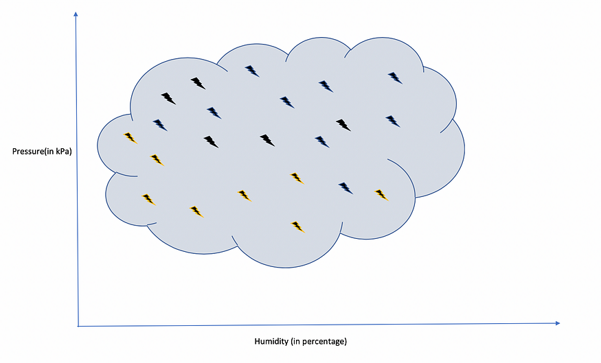
Humidity is measured in percentage and pressure in kilopascal.
If one uses his intuition, that if humidity is higher than a certain threshold, then the probability of rain is high. So what exactly he is doing is just dividing the data set in two halves based on humidity.
x1 = 70 (say ) be the threshold .

Now we have some rule which splits the data set and creates two regions R1 and R2. We made some progress in classifying the points. The very next question which pops up is how good is our split.
There can be multiple ways to validate our decision. One of measure can be as simple as to count the proportion of miss-classified points in each region. The definition of misclassified points is that all points whose labels are different from region labels are classified wrongly. In our scenario, R1 is for rain, so all non-rain points are considered as misclassified. Similarly, R2 is for no rain, so all points corresponding to rain are wrongly classified.
Let us call this measure as M(R), where R denotes the region.
for R1 , M(R1) = 1/7
similarly for R2 , M(R2) = 8/15
The overall measure can be any combination of M(R1) and M(R2); one way is to take the mean. The only problem with this approach is that it doesn’t take the volume/density of the region into account. So a better way to combine them is via weights, proportion to the size of each region.
Calculation of M(R)
R : Overall region , n points i.e U+007CRU+007C = n
U+007CR1U+007C = n1 , U+007CR2U+007C = n2
n1 + n2 =n
R = R1 U R2
w1 = weight of region R1
w2 = weight of region R2
w1 + w2 =1
M(R) = w1*M(R1) + w2*M(R2)
= n1/(n1 + n2)*M(R1) + n2/(n1 + n2)*M(R2)
In our case n1 = 7 , n2 = 15 ,M(R1) = 1/7, M(R2) = 7/15
M(R) = 7/22*(1/7) + 15/22*(8/15) = 0.41
Lesser the M(R) better the model.
The other interpretation of M(R) is in terms of an intraclass and inter-class concept of clustering where high inter-class and low intraclass variance leads to well defined separated clusters.
Let’s move on and further subdivide the two regions based on pressure value.

Now it looks somewhat better than the previous split, the one based on humidity only. I leave it to the reader to calculate M(R) value and validate the above argument.
This entire experiment of iteratively splitting parameter space into smaller spaces is what we called a decision tree approach for classification.
Formally, a decision tree is a tree-based algorithm of decisions and their outcomes.
The node represents the evaluation, outcome of each evaluation as a branch, leaf nodes as a class. The entire path from the leaf node to each internal node and finally root node as the decision/classifying rule.
The graph notation of the above experiment is in the below image.

It is a good time to know each element of the decision tree before deep dive.
- Root Node: The one at the top that contains an entire sample.
- Branch Nodes / Sub Nodes: Nodes obtained after the split.
- Parent-Child: The node which splits is called the parent and the branch nodes as children.
- Split Value: The value at which evaluation happens to split parents into children. The process to divide is known as splitting.
- Leaf Nodes / Terminal Nodes: The child node with no children.
- Sub Tree: Any set of branch nodes with at least one leaf node.
- Edge: The path between any two nodes, a line joining two nodes.
- Depth of node: The number of edges to reach the root node from that node.
- Height of node: Maximum number of edges to reach a leaf node.
- Pruning: The process of trimming off a portion of the tree that has less predictive power.

- Depth of root is 0; height is 3 since the max step is three, to reach a leaf 8 in this case.
- The height of any leaf node is 0.
- The depth of node 3 is 1 and height 2.
- The depth of node 4 is 2.
We have discussed one metric to decide the goodness of split. Next, we discuss some other metrics such as Gini Impurity, Entropy, Chi-Square, Variance.
Other Metrics
Gini Index (GI) :
Gini Impurity of a node is the probability that any randomly chosen point in that node is misclassified if it is assigned the label of that class.
Let pi: the probability of point with label i
GI(point) = pi*(probability it belongs to label other than i) =pi(1-pi)
Suppose there exists M classes/label.
GI(node) = sum of GI(all points) = sum of pi(1-pi) for all i belong to {1,2,..,M}.
GI(node) = 1- pi**2 — p2**2 — … -pM**2
for binary classification ;
GI(node) = 1 — pi**2 — p2**2, where p1 is the probability of yes, p2 probability of no.
Consider a node (S) with binary value say yes or no.
S= { Yes, No, No, Yes, Yes, Yes, Yes, No, No }
p1 = prob of Yes : #Yes/(#Yes + #No)
p2 = prob of No : #No/(#Yes + #No)
# denotes cardinal or count
since p1 + p2 = 1
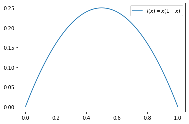
GI = 2p1*p2
if we want high p1, then cases of No should be quite low and vice versa. This symmetrical measure serves our purpose.
We see from the above plot that for p1 = p2, it is optimum.
Overall, GI is w1*G1(node1) + w2*G1(node2), where w1 and w2 are weights of that node.
Lower the GI better the split.
Python implementation of GI
Let’s calculate GI in our rain prediction problem.
Split based on humidity :
w1 = 7/22, w2 = 15/22
for node 1
p1 = 6/7 ,p2 = 1/7
g1 = 0.24
for node 2
p1 = 8/15,p2 =7/15
g2 = 0.5
GI(humidity) = 0.42
Split based on pressure:
w1 = 14/22, w2 = 8/22
for node 1
p1 = 13/14 , p2 = 1/14
g1 = 0.13
for node 2
p1 = 1/8,p2 =7/8
g2 = 0.22
GI(pressure) = 0.16
Therefore split should be based on pressure.
2. Information gain based on entropy
Entropy is defined as the expectation of self-information I(x)

Consider a sample we assume there is an unknown process(random variable) that generates this sample. The maximum likelihood principle obtains the parameters that maximize the sample and process.
If one observes a data point with the unlikely value, we called that self-information as it gives more information about the random variable.
The most real example can be tossing a coin; if you know it is biased towards the tail, the self-information will be 0 as there is no information obtained. Similarly, for the unbiased coin, it will be maximum, i.e., 1.
Information gain = 1- Entropy
In terms of probability E(node) = -p*log(p) -q*log(q) , p+q = 1
Here also entropy for each node is evaluated, and then the weighted average is taken as entropy to decide the split.
3. Chi-Square :
Yet another measure to evaluate split based on the statistical significance of parent-child node
C(node) = (Actual — Expected)**2 / (Expected)**2
The calculation is there in my previous blog of the goodness of fittest.
4. Variance :
So far, the measure we have discussed is for categorical variables; in case of a continuous variable, we use variance. The method is the same, calculate variance for each node, and then use the weighted variance to decide the split.

The different algorithm of decision tree use different measures.
Model Complexity
So now, we have understood how to split the root node into branch nodes. If we continue doing this process at the end, we end up homogeneous leaf nodes as a class label. There is a high risk of overfitting, and complexity also increases to overcome this; we start removing nodes that don’t contain sufficient information. This process is called pruning of a tree, which we evaluate on the cross-validation set.
The other way to overcome overfitting and model complexity is to play around with different parameters of the classifier.
- Max depth of the tree. max_depth int, default=None
- Min no of points in a leaf. min_samples_leaf int or float, default=1
- Max, no. of leaf nodes. max_leaf_nodes int, default=None
- Min no of points in a node to split. min_samples_split int or float, default=2
- Max features. max_features int, float or {“auto”, “sqrt”, “log2”}, default=None
- Min decrease in impurity for the split. min_impurity_decrease float, default=0.0
- Other factors depend on the use case.
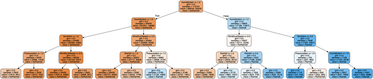
Python Implementation
Data Set: Snapshot of rainfall data set.

target = [ NoRainfall , Rainfall ]
We have done EDA and data preprocessing, you can see in the previous blog of where we implemented logistic regression. So, for the time being, you can assume this data is clean.
Visualization
Comparison between Gini and entropy for this data set.
Like all estimators in the sklearn, DecisionTreeClassifier also has a predict and score method.
As we know, the default criterion is Gini, how about using an entropy.
Gini based model Score: 0.834
Entropy-based model Score:0.836
In this data set for the same hyper-parameter, entropy is performing slightly better than the Gini one.
The other metric to measure a classifier is there in my previous blog.
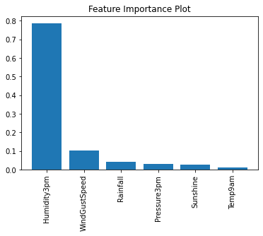
Feature Importance, and its calculation
Once the model is trained, the next task is to figure out essential features governing the model. The importance of features is quite useful to convince others about our model and also for inference purposes. The insight from the data and helps in the process building of any service.
Hyper-parameter tuning
There are different techniques for tuning the hyper-parameters; it in itself is a whole new paradigm. There can be a separate blog on how to optimize your model hyper-parameter.
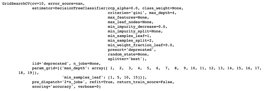
In this talk, we will be using Grid-searchCV, it is just an exhaustive search over given parameters of the estimator, DecisionTreeClassifier in our case. It uses a cross-validation technique over the grid search to come up with optimum parameters based on the scoring method provided.
print(grid.best_score_)
print(grid.best_params_)
print(grid.best_estimator_)0.8403836694950619
{'max_depth': 8, 'min_samples_leaf': 10}
DecisionTreeClassifier(ccp_alpha=0.0, class_weight=None, criterion='gini',
max_depth=8, max_features=None, max_leaf_nodes=None,
min_impurity_decrease=0.0, min_impurity_split=None,
min_samples_leaf=10, min_samples_split=2,
min_weight_fraction_leaf=0.0, presort='deprecated',
random_state=None, splitter='best')
So we see the best parameters are {‘max_depth’: 8, ‘min_samples_leaf’: 10}, and accuracy 0.84, which is better than the vanilla model.
I leave it for the readers to include some other hyper-parameters like criterion,max_leaf_nodes,min_samples_split,max_features,min_impurity_decrease, and fine-tune the model.
Pruning
The process of trimming off a portion of the tree which has less predictive power.
As mentioned above, pruning is used to generalize the model to unseen data, that is, reduce overfitting and complexity also. The other way to understand this phenomenon is that one should know when to stop, but for practical purposes, we never knew how adding / deletion of a single node can change the score drastically. The above phenomenon is also known as the Horizon effect.
In our case, train accuracy was 0.8349 and test accuracy as 0.8344, which is quite similar, so there is no case of overfitting.
Nevertheless, let’s see how pruning works and its python implementation.
There are different ways, either pre pruning or early stop U+1F6D1 , which has its own challenges as mentioned, so here we will post prune.
We will discuss one such post pruning implementation as mentioned L. Breiman, J. Friedman, R. Olshen, and C. Stone paper.
Minimal Cost-Complexity Pruning
Minimal Cost-Complexity Pruning is intuitively a way of adding penalties for an increase in the split.
We define a cost C(α, T) for a tree T, where α ≥0 is known as the complexity parameter.
C(α ,T) = C(T) + αU+007CTU+007C ,
C(T) : Total misclassification of leaf/terminal nodes
U+007CTU+007C: Number of terminal nodes in a tree T.
To move further let’s try to understand C(T)

c(t): the probability of misclassification for points in node t.
Probability of misclassification of the whole tree: use the total probability formula.

The miss-classification rate of parents is always greater than the weighted sum of the child. So if we keep on splitting, misclassification decreases, which eventually leads to overfitting.
Given a tree T < T_max,
T_max: max possible tree.
If α=0: largest tree selected
for α tending to infinity single root node tree.
To get optimal T(α), we need to minimize C(α, T).
C(α ,T(α)) = min (C(α ,T)) for all T < T_max
min exists since we will have only finitely many values of T.
For optimum
- C(α ,T(α)) = min (C(α ,T)) for all T < T_max)
- C(α, T) = C(α ,T(α)) ===> T(α) ≤ T , else there exists a bigger tree.
for a single node we will have C(α ,T) = C(T) + α
Consider a tree (branch) whose root is t and denote it by T_t
C(T_t) ≤ C(t) , from equation of inequality of parent child.
α_opt is the value where equality holds that is
C(T_t) = C(t)
C(T_t) + αU+007CT_tU+007C = C(t) + αU+007CtU+007C = C(t) + α
α(U+007CT_tU+007C-1) = C(t)-C(T_t)
α_opt = C(t)-C(T_t) / (U+007CT_tU+007C-1)
Weakest link: Any non-terminal node with the smallest value of α_opt
We prune the weakest link till α_opt ≥ ccp_alpha parameter.
Python Implementation
Decision Tree Classifier has method cost_complexity_pruning_path(self, X, y, sample_weight=None) to compute the path of pruning. It returns for each step the optimum alphas and the corresponding total leaf impurities.
Here I am using a sklearn visualization script for pruning in our example.

Number of nodes in the last tree is: 3 with ccp_alpha: 0.061183857976855216

We wrap up pruning with one last observation, which is between accuracy and alpha.
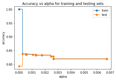
Initially, test acc was around 0.78 and train 1, as alpha increases equilibrium is attained.
In this blog, we learned how the decision tree works, python implementation, hyper-parameter tuning, and pruning.
I hope you enjoyed it U+1F60A !! U+1F942
Join thousands of data leaders on the AI newsletter. Join over 80,000 subscribers and keep up to date with the latest developments in AI. From research to projects and ideas. If you are building an AI startup, an AI-related product, or a service, we invite you to consider becoming a sponsor.
Published via Towards AI
Related posts
Popular posts

 for 2021")


Updates

Recent Posts