Baseball Pitch Prediction

Last Updated on December 18, 2020 by Editorial Team

Author(s): Shafin Haque

Predicting the next pitch in baseball with machine learning

Introduction

Dodger’s shortstop Corey Seager is up to bat with two outs in the ninth inning. Fastball inside, he makes contact… grounder to second, and he’s out. And the Astros win the 2019 World Series in 7 games.

It was eventually found out the Astros were using cameras to figure out the next pitch. A batter knowing the upcoming pitch gives the team a huge advantage, and some of the Astros’ coaches and players were heavily penalized. However, this incident left me wondering if there could be a way to predict the next pitch without “cheating.” I decided to use Machine Learning and Data Science to predict the next pitch based on the current game scenario. By this, I mean all factors that are numbered and available for all to see, such as the strike count, ball count, runners on base, and more.

Data Cleaning

The data I used can be found on Kaggle. The overall dataset contains eight comma-separated value(CSV) files, containing data from the MLB seasons 2015–2018. However, I focused on two of the files, pitches and at-bats. The pitches CSV file contained 40 data columns, and the at-bats had 11. Both of them had data values that I would need, so I decided to merge the files. The merged file contained 51 variables, but the majority of them were not needed. Many different columns were describing the actual pitch, as in the movement of the ball with coordinates. These would not help, as the pitch type would serve just as good as all these columns combined.

At first. I simply looked through all of the variables and thought of which could influence a pitcher’s decision for their next pitch based on my knowledge.

I decided to make a simple data frame, containing only a few variables and could be used for a basic model. I settled on keeping the strike count, ball count, the pitch number and adding two new variables to the data. The first variable was similar to the pitch_type variable. However, it was binary. Any 4-seam, 2-seam, or cutters would return a 1 for this variable (classifying it like a fastball), and any other pitch type would produce a 0. The second new variable displayed the previous pitch. However, it was not binary. To make means simpler, I combined the 4-seam, 2-seam, and cutter as fastballs, and the curveball and slider into 1 pitch type.

The next data frame contained those variables in addition to if runners were on base, the pitcher’s id, the pitcher stance, and the batter stance. I thought these variables would allow the model to perform better. Lastly, I created the data frame for multi-classification, in which the fastball variable would contain all of the pitches, instead of it being binary in the previous data frames. When first creating this data frame, I wasn’t sure if it would be possible to predict the exact pitch type. After categorizing some pitch types together, I settled on four different pitch types, FF(4-seam, 2-seam, or cutter), CU/SL(curveball or slider), CH(changeup), or other. Data cleaning, with the exception of merging, was done in R, with tidyverse.

Data Visualization and Statistics

Pitch Type Graph

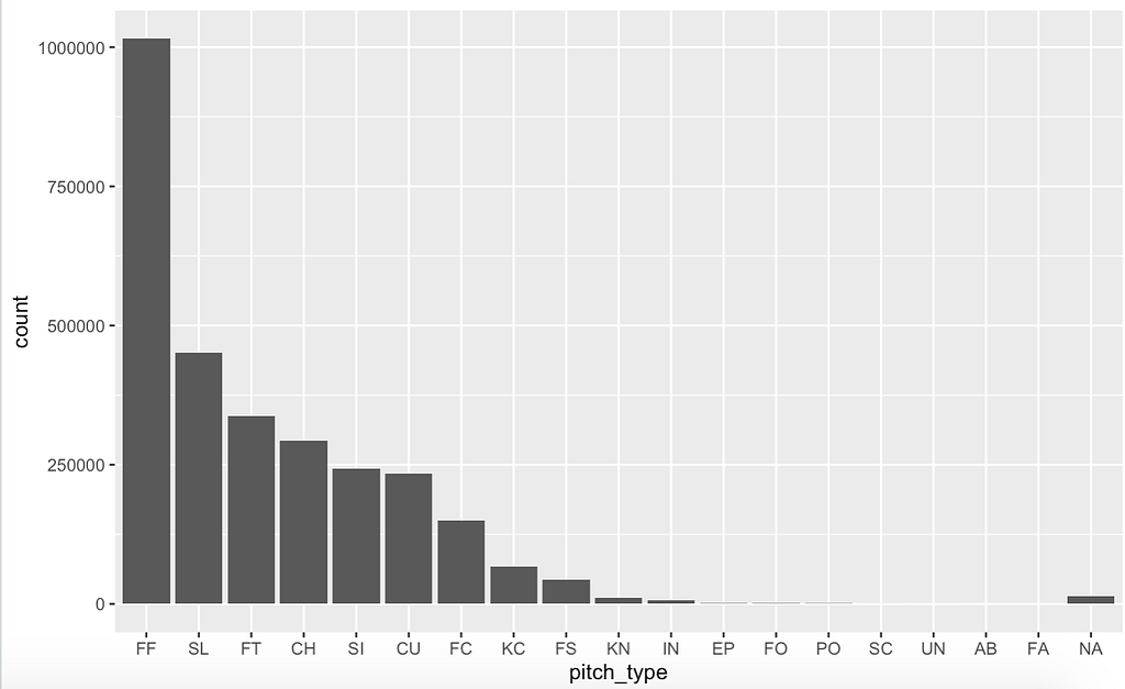
I had one graph in mind when first gathering the data. I wanted to see the amount of each pitch thrown. This bar graph shows the count of every type of pitch throughout all 3 seasons. This shows us that fastballs are by far the most common pitch and account for a bit less than half of all pitches.

Variable Correlation Heat-map

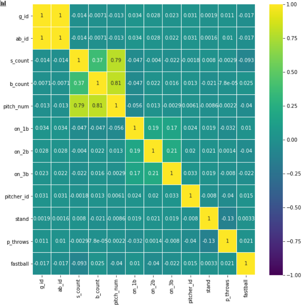
This correlation heat-map displays the correlation between the variables. The correlation ranges from -1 to +1. The lighter the color, the higher the correlation. This will allow us to see which variables are necessary and if we can remove any. Because we want to predict the Fastball variable, we need to look at “fastball” and the values from the other variables. In this heat-map, we must focus on either the bottom-most row or the rightmost column as they are the same. The heat-map did not give much information as to which variables are helpful in predicting the pitch, which just tells us it is going to be very hard to predict at a high rate. You can also see some of the values are very high, and the reason for that is because they are directly correlated. For example, the pitch number of the at-bat would have a direct correlation with the strike and ball count.

Model Building

The two first models I created were a generalized linear model(GLM) and a support vector machine(SVM). I created both of these in R. These models predict the pitch with binary classification(1 for a fastball, 0 for others). I used the strike count, ball count, pitch number(of the at-bat), the last pitch if there are runners on any base, batter stance, pitcher id(every pitcher is given an id), and pitcher stance.

A GLM is different from a normal linear regression model because it ‘generalizes’(hence the name) linear regression by allowing the linear model to be related to the response variable via a link function and by allowing the magnitude of the variance of each measurement to be a function of its predicted value. The result outputs a value between 0 and 1. In our case, if it’s 0.5 or lower, it’s not a fastball, and if it’s 0.5 or higher, it is a fastball. When starting with the GLM, I used my data frame, which contained data for 2018 only. I did not split the data into testing and training. However, I fit the model to all the data and created a visual to go along with it. I had no idea what accuracy to expect, and the model ran extremely fast. After running the model, it gave me an accuracy of 60.5%.

I was quite surprised. It was a very basic model and did much better than someone guessing randomly, which would give you around a 47% accuracy as there are more fastballs than there are other pitches. However, there are no hyper-parameters you can tune in a GLM model, so on to the SVM.

A support vector machine(SVM) takes all of the data and creates optimal boundaries between outputs. The model will do complex data transformations and separate your data into different groups(for this project it’s two groups, fastball, or not). The output will be between -1 and 1. 0–1 range will return a fastball and -1–0 range will give not a fastball.

The SVM took quite a while to fit to 1 year’s worth of data, so I settled for the first 100 games in the 2018 season for a baseline. With only 100 games, the SVM model was able to predict the pitch at an accuracy of 61% exactly. With more data, I’m not sure how much more accurate it would be, but I don’t think it would be much more accurate, as the GLM’s accuracy with 100 games is 60.3%, and its accuracy with 1 season is 60.5%. However, this was with the default values of the model. I tuned the hyper-parameters of the SVM and was able to come to a final accuracy of 66.1%. This was quite impressive considering it trained off of 100 games only, but I was skeptical of the accuracy. I believed if I split the data into test and train, the model’s test accuracy would be much lower, and I thought that with more data the accuracy would go down, as it’s over-fitting to the 100 games.

However, I thought I would be able to create an even better model with a Random Forest model. I decided to create this model in R as well. A Random Forest Classifier creates decision trees on data samples and then gets the prediction from each of them and finally selects the best solution by means of voting. Another issue this model faced, similar to the SVM, was that it took a long time to run the model, so I could only test accuracy on 100 games. The base model’s accuracy was around 52%. For the final model, I decided to do a train/test split, and after tuning hyper-parameters, the testing accuracy was around 54%.

I decided to take both the SVM and random forest to Python to see if it would make fitting to 1 season faster.

This time around for the SVM model I split the data into training and testing in a 70/30 ratio. Initially, when trying to fit the model I ran into a problem, as some of the variables had string values, and Python models do not allow strings. To fix this, I had to use one-hot encoding for the pitcher/batter stance, and the last pitch variable. The default SVM model training off 100 games in the 2018 season produced an accuracy of 52%. This was pretty miserable, but I had confidence in tuning the values.

After tuning the Python SVM’s hyper-parameters using a grid search and testing many different costs, gammas, and kernels I was able to get a final accuracy of 67.35%. I was pretty surprised by the huge jump in accuracy from the starting model to the final model. I think this was a great start to the models, and if I ran it with all 3 seasons, it would maybe even get to 68%. However, I wasn’t completely satisfied with this result. I wanted to reach at least 70% accuracy, maybe even 75%, if that’s even possible, so I decided to try two more models.

After finishing the SVM I moved back to the Random Forest, but this time in Python. Testing the base random forest model gave me an accuracy of 60.91% on the testing data. This was much better than the base model of the SVM which had an accuracy of around 52%. This gave me a lot of hope for accuracy after tuning. However, my hope was not fulfilled. The tuned model had an accuracy of 62%.

From here I shifted gears to my final model, a neural network. I did not have very much experience with neural nets so I had to read up. I created a basic model with 3 layers which had 8,8, and 1 neuron with the activation of a relu. This was just a test model and when tested on 100 games worth of data with 4 epochs it performed quite terribly. After this, I decided to tune it with 3 layers going from 12,8,1 neurons, however trying multiple optimizers with the grid search function. Despite much testing and tuning the neural net could never perform well and only got to around 52%. Thus, I decided to use the SVM for the final model.

Because the final app was created in R to make means simpler for the app backend, I decided to go back and create the SVM in R with the same hyper-parameters as the python model. Essentially I trained and tested the model in python, then created a final model training it on all 3 seasons in R.

The Dashboard/Application

When creating the dashboard I decided to keep it simple. Have some sort of way to have a user input the variables and when they click the button it will display text about whether or not the pitch was a fastball. Creating the front end was quite easy as it was just a couple of numeric inputs or text inputs. I thought the backend would be easy, but it was actually quite hard. I saved the model as an RDS file, which can be practically any object in R, and loaded it up in the app. I then took the user’s inputs and put them directly through the model. When I tried this it gave an error that said “contrasts can be applied only to factors with 2 or more levels”. I was quite confused until I realized that the reason this was happening was that the model had no comparison to other data. The only data it was fed was the user’s inputs. To fix the issue I took the 100 game dataset and only kept all of the different unique data points. I assumed this would have the same amount of unique data points as 1 season or more, so there should be no issue here. I then ran the model on the user inputs, as well as the unique dataset so that it had a comparison. This fixed the issue and displayed whether the pitch would be a fastball or not properly. You can try the app on R Shiny

Final Thoughts

When first diving into this project I thought I would be able to create an application that could predict the next pitch of a baseball at a pretty high accuracy rate. When first creating the models and seeing accuracy rates of around 50–60% with 100 games of data, I still thought I could get maybe a 70+ accuracy rate by tuning the model values and using more data. However, I now realize that it’s simply not possible. As Hank Aaron once said, “Guessing what the pitcher is going to throw is 80 percent of being a successful hitter. The other 20 percent is just execution.” Predicting the pitch coming at you can make you an infinitely better hitter, and because of this, the task at hand was a lot harder than originally thought. Although I may not have been able to create a project at the caliber I wanted, overall I still think the final product was great and was a great learning experience for me.

Future of the Project

I am currently working on creating a similar model and app, however, instead of predicting the pitch, it will suggest the pitch that will have the highest chance of a strike/out. In terms of this project, I think it’s finished. There isn’t that much more I can do to make the project better and once I finish the other app I could try to merge them into one which would make for a single cool app.

Github Repo: https://github.com/ShafinH/Pitch-Prediction

Demo App:

Baseball Pitch Prediction

Baseball Pitch Prediction was originally published in Towards AI on Medium, where people are continuing the conversation by highlighting and responding to this story.

Published via Towards AI