


An Overview of Multilabel Classifications
Last Updated on July 20, 2023 by Editorial Team
Author(s): Abhijit Roy
Originally published on Towards AI.
Machine Learning
How can we classify an instance as multiple classes?
We are very familiar with the single-label classification problems. We mostly come across binary and multiclass classifications. But, with the increasing applications of machine learning, we face different problems like movie genre classifications, medical report classification, and text classification according to some given topics. These problems can’t be addressed using single-label classifiers, as an instance may belong to several classes or labels at the same time. For instance, a movie can be of Action and Adventure genre at the same time. This is where multilabel classification steps in. In the article, we will go through some common approaches to handle multilabel problems, and in later parts also look at some applications.
Before we jump into approaches, let’s take a look at the metrics used in such problems.
Metrics
In binary or multiclass classification, we normally use Accuracy as our main evaluation metrics and additionally F1 score and ROC measures. In multilabel classification, we need different metrics because there is a chance that the results are partially correct or fully correct as we are having multiple labels for a record in a dataset.
Depending on the problem there are 3 main types of metrics classes:
a. Evaluating Partitions
b. Evaluating Ranking
c. Using label Hierarchy
Partitions
To capture the partial correctness, this strategy works on the average difference between the actual label and the predicted label. We pick up samples from our dataset and predict those samples using a model. We obtain the difference in actual and predicted labels of the samples one at a time and then find the average differences over all samples. This approach is called Example-Based Evaluation.
Another method is predicting all the test-data set, and evaluating the difference label-wise, i.e, considering each label of the result as a single vector and finding the difference between the predicted values and the actual values for a particular label. Once we find the difference for each label. We take an average of the errors. This is called Label-Based Evaluation.
So, we can say Example-based is a row or sample wise approach to find the difference, it treats the all the predicted labels of a sample as a whole, finds the difference for one sample at a time, whereas, for the Label-based, it is a column or label wise approach, it treats each label as a whole, i.e, the values of all the samples for that particular label is considered. We find the difference between the predicted and actual value for that label and average overall labels.
This approach of Label-based to treat each label independently fails to address the correlations among the different class labels.
1. Example-Based Metrics
- Exact Match Ratio: This approach doesn’t consider the partially correct, regarding them as incorrect. So, it presents the multi-label prediction as single-label predictions. The main issue is it does not distinguish partially correct and fully incorrect. In the equation below, Y is the actual labels vector and Z is the predicted labels for sample ‘i’, summing over all ‘i’ from 1 to n samples. It considers only if both the prediction and actual label vectors are completely the same.
MR = np.all(y_pred == y_true, axis=1).mean()
- 0–1 Loss: The approach is similar to Exact match ratio and is given by
1-Exact Match Ratio
- Accuracy: Normally accuracy is given by Accuracy= TP / (TP+FP+FN+TN). For multilabel, the definition is given as:
In the equation, the Z is the predicted label vector and Y is the actual label vector for sample i. Now, by definition, a result is said to be True Positive, if the predicted label and the actual label is the same. Here, we take the intersection of the two vectors, so, the resulting vector has only those labels as 1, where both the actual and predicted vectors were true or 1. On taking the Mod value of the vector, we get the numerical value.
Say, (0,0,1,1,0)->Z is the predicted vector for a sample and (0,1,1,1,0)->Y is the actual vector, So mod(Intersection(Y,Z))=2.
For union, mod(Union(Y,Z))=3. Overall partial accuracy=⅔ =0.67 for that particular sample because it correctly classified, 2 out of 3 labels. If it wrongly predicts a label also the union increases, i.e, the denominator increases, penalizing the accuracy. Then we find this score for each sample and average it over all samples in the set.
def Accuracy(y_true, y_pred):temp = 0for i in range(y_true.shape[0]):temp += sum(np.logical_and(y_true[i], y_pred[i])) / sum(np.logical_or(y_true[i], y_pred[i]))return temp / y_true.shape[0]Accuracy(y_true, y_pred)
- Precision: By definition, Precision measures how many of the samples predicted as Positive class is actually positive. It is given by TP/(TP+FP). False Positives are the samples that are wrongly classified as the model as true. The score is modified as:
The numerator gives the labels as 1 for which both the predicted values and the actual values are both true. So, the True Positives. The denominator gives all the labels as 1, whose predicted values are 1. So, it contains both TP and FP. Thus for a particular sample, we obtain the value taking modulus and average it out for all samples.
(0,0,1,1,0)->Z is the predicted vector for a sample and (0,1,1,1,0)->Y is the actual vector, So mod(Intersection(Y,Z))=2.
mod((Z))=2.
Precision=1 for the sample, as there are no false positives here
def Precision(y_true, y_pred):temp = 0for i in range(y_true.shape[0]):if sum(y_true[i]) == 0:continuetemp+= sum(np.logical_and(y_true[i], y_pred[i]))/ sum(y_true[i])return temp/ y_true.shape[0]
- Recall: According to the definition, Recall is given by TP/TP+FN i.e, it determines how many of the samples which were actually true in the dataset, are predicted as true by the model. It is modified as:
So, the numerator gives True positives as we have seen, the denominator gives all the labels as 1, which is actually true for a given sample.
(0,0,1,1,0)->Z is the predicted vector for a sample and (0,1,1,1,0)->Y is the actual vector, So mod(Intersection(Y,Z))=2.
mod((Y))=3.
Recall=0.67 for the sample, as there 1 false negative. We take the average over all the samples.
def Recall(y_true, y_pred):temp = 0for i in range(y_true.shape[0]):if sum(y_pred[i]) == 0:continuetemp+= sum(np.logical_and(y_true[i], y_pred[i]))/ sum(y_pred[i])return temp/ y_true.shape[0]
- F1 Score: It is given as the harmonic mean of Precision and recall. It can be thought like, calculating the F1 score for a sample and then averaging it over all samples. It is given by:
- Hamming Loss: The Hamming Loss tries to account for any label that is wrongly predicted by the model for a particular sample that is, it considers both False Positive and False Negative cases together. It calculates a score for each sample on this basis and then finally finds a summation over all the samples. It is given by:
So, here k is the number of classes or labels for a sample i. ‘I’ is the indicator function. First, for sample ‘i’, the equation iterates over all the labels ‘l’ for l in 1 to k. It then tries to find a label ‘l’ for which the predicted value does not match the actual value. It sums all the errors and divides by the number of labels.
(0,0,1,1,1)->Z is the predicted vector for a sample and (0,1,1,1,0)->Y is the actual vector.
For the given sample, for label class at index 0, they match so, error=0, at the second index a mismatch is found, as l for Y=1 and l for Z=0. So, logical and gives 1 for the second condition in the equation. So, summing up, the whole sample gives a hamming loss of ⅖, as there are 2 mismatches on 5 labels. This score is taken average over all the given samples.
Hamming loss =0 means no errors.
def Hamming_Loss(y_true, y_pred):temp=0for i in range(y_true.shape[0]):temp += np.size(y_true[i] == y_pred[i]) — np.count_nonzero(y_true[i] == y_pred[i])return temp/(y_true.shape[0] * y_true.shape[1])Hamming_Loss(y_true, y_pred)
2. Label-Based Metrics
Label based measures all the labels separately. If there are k labels it considers the evaluation as evaluation of k different binary classification results. So, any units or procedures for measuring accuracy, precision, recall, F1-score can be used without any modification here for each label. Then we take the average of the scores over all the labels. There are majorly 2 methods:
- Macro-Averaged Measures: It is according to the above logic, i.e, first, the measures of each label is calculated. Then we take the average over all the labels. It is given by:
For each label, the precision, recall, and F1-score are calculated and then we take the average over the entire number of classes or labels (k).
- Micro-Averaged Measures: It takes the True Positive, False Positive, True Negative, and false negative for each label separately and then calculates the precision, recall, and F1 scores. It is given by:
Here n is the total number of samples. There exist k class labels., Y represents the actual set of output labels and Z represents the predicted set of output labels. The difference here is the summation over all the labels is the outer summation. The inner summation sums over all the samples from 1 to n. YiZi is the true positives for ith sample for the jth label and so on.
For 2 labels, Micro precision is given by: (TP1+TP2) / ( TP1+TP2+FP1+FP2)
For 2 labels, Micro Recall is given by: (TP1+TP2) / ( TP1+TP2+FN1+FN2)
Dataset Properties
Before starting operations on a dataset, we need to analyze the data and its distribution. For multilabel it is done based on:
- Distinct Label Set(DL): It is given by the total count of the number of distinct label combinations observed in the dataset. It accounts for the distribution of different labels.
- Label Cardinality(LCard): It is given by the average number of labels per example. It accounts for the distribution of samples as well as labels.
Multi-Label Learning
There are two types of algorithms to handle multilabel classification:
- Simple Problem Transformation Methods
- Simple Algorithm Adaptation Methods
Problem Transformation Methods:
The methods convert multi-label problems to single-label problems and then use binary classifiers and other available methods to classify. Notable methods in the category are:
- There are some simple transformation methods. Let’s discuss some of them.
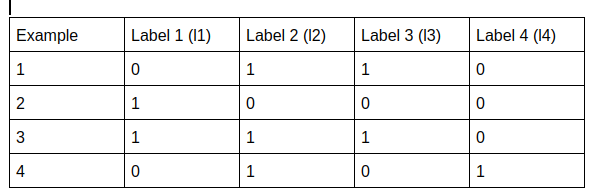
We are ignoring the features for the moment
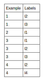
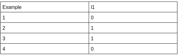
- Copy Transformation: It creates new examples for each sample having multiple labels. So, It copies the features, for each sample and considers each label once. The above table modifies to:
- Dubbed Copy Transformation: It is similar to copy transformation, the difference is here along with the labels a weight is also assigned.
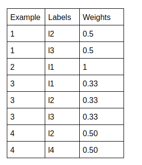
The weights are actually 1/(Number of labels having value 1 for the sample).
- The next method selects one label out of the set of labels which have the value 1 for a particular sample. Based on the process of selection, there are 3 choices
- Select Max
- Select Min
- Select Random
- Ignore: It just ignores the multilabel data. So, here the final dataset will have only the example 2.
- Label Powerset(LP): It creates new labels for distinct combinations of labels. Thus it creates a multiclass classification. For our dataset, it is modified as:
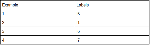
Where l5 is the combination of l2 and l3, and so on. The upper bound of the number of labels that can be created is given by min( n, 2^k) where n is the number of examples and k is the number of labels. The 2^k considers all given combinations that can be formed using the basic k labels given. So, it is the worst case or n i.e, the number of examples, because you can’t have 2⁴= 16 combinations if you have only 10 examples.
The problem with the approach is that it creates highly imbalanced sets because some combinations may occur a very less number of times or maybe even once or twice, so those new levels will be a lot underrepresented.
To solve this problem, a Pruned problem transformation is used, it takes in a user threshold say a label has to appear at least 4 times in a given example set. If a label is not found 4 times the label is ignored.
- Binary Relevance: This method is most commonly used. It creates k datasets one for each label. So, it basically transforms a k class multilabel classification into k disjoint binary classification. Our dataset gets modified to:
After the conversion results for each of the binary classifications are obtained and then we take the union of the results for each sample and get the results for our multiclass classification. This approach is criticized because of assumptions based on the independence of the labels. It uses k different models for each class, so each prediction is independent of one other.
- Ranking by Pairwise comparison: It creates kC2(combination) datasets from k given labels. So, it picks label Li and label Lj, such that i<j<k combine them together to form a new label. Each dataset retains an example from the original set if the example belongs to at least any one of the set but not both.
Algorithm Adaptation methods
The methods try to modify the definition of common algorithms like SVMs and decision trees which are used for single-label classification, in a way that they are fit to work for multilabel classifications.
The loss function Log Loss or Binary cross-entropy which is the most used loss function for classification problems is modified to:
where, P(λj ) = probability of class λj. So, it calculates the loss for each label, similar to how it does for a normal single-label binary classification, and later sums all the losses for all the labels to give the final loss.
There are mainly three ways:
- Tree-Based Boosting: The algorithm focuses to modify the AdaBoost algorithm used in Gradient boosting of trees to produce results for multiple labels data. There are two types of modifications: AdaBoost.MH which tries to classify through minimizing hamming loss and AdaBoost.MR.
Adaboost algorithm generally works on three main points which are different from the random forest algorithm:
- The Adaboost algorithm works on stemple or weak decision tree learners. They have one root i.e, they can only use one of the features at a time to predict the labels. They are not full-grown trees as we use in the random forest algorithms.
- In AdaBoost, different trees in the forest get different weights assigned i.e, all the trees don’t have the same say or influence over the final result or predictions unlike random forests, where all the trees have equal weightage to decide the results.
- The trees in Adaboost learn from mistakes the previous ones. So, they are dependent, and dependent on the order the trees are formed, unlike random forests the trees are independent of each other.
2. Lazy Learning: Lazy learning is based on the K Nearest Neighbour approaches. They can work on both problem transformation and algorithmic adaptation approaches. For problem transformation, the most commonly used approach for Lazy Learning is BR-KNN. It is a procedure where binary relevance is used to transform the multi-label classification into a single label classification and thereafter KNN is applied.
3. Neural Networks: Back Propagation algorithms of the neural networks have been modified to suit a multi-label problem. The loss function actually is modified to take into account the errors across multiple labels. The approach is called BP-MLL.
4. Discriminative SVM Methods: The common SVM method uses a binary relevance method to obtain the result for the binary classification of each of the k labels individually in the first step. Then it extends the dataset by k additional features which are actually the predictions of the binary classifiers in the first step. In the next step, ‘k’ new binary classifiers one for each k label. The new classifiers train on the extended datasets to take into account the dependencies of the labels. There are other approaches like BandSVM.
Other Available Methods
- One-Vs-Rest: This approach is very similar to the binary-relevance approach. It treats all the k labels to be mutually exclusive and trains a different model with the same hyperparameters for each of the k labels. So, the models are trained independently and do not take into account the correlations among the different labels. It creates independent binary classification problems.
- Classifier Chains: They take into account the dependence or correlation between the k labels. It creates k binary classifiers for k labels. The first binary classifier takes up the data set and predicts the first label. Say the prediction is C1. For the next classification label, a second binary classifier is used. For the second we pass the feature set plus C1 i.e, the classifier output for the first classifier output. Say, it gives C2. For the third label classifier, we feed, all features+C1+C2. So, for the classification of the nth label, we extend the feature set by n-1 features which are actually the predicted labels of the previous n-1 classes.
Application
Now, let’s look at the applications of the above algorithms in python.
For the application, I have used kaggle’s Toxic Comment Classification Dataset available here. This is one of the most commonly used datasets for the purpose. Let’s continue.
Data Visualization
On visualization, the data looks like the following:

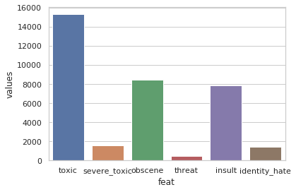
It has 6 classes in which each statement has to be classified. The classes are:
Index(['comment_text', 'toxic', 'severe_toxic', 'obscene', 'threat', 'insult',
 'identity_hate'],
 dtype='object')
The classes are not very well balanced though. The ‘toxic’ class is represented at a very high rate compared to the others.
Now, one thing to notice here is the correlation of the 6 labels with one another.
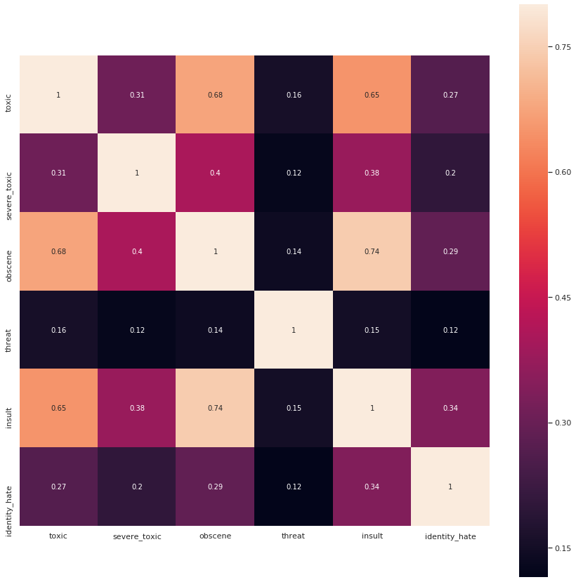
The above diagram shows the correlations among the labels. We can observe the ‘obscene’ class and the ‘toxic’ class will have a high correlation.
Data Preprocessing
The ‘comment_text’ column will be our feature set.
0 Explanation\nWhy the edits made under my usern...
1 D'aww! He matches this background colour I'm s...
2 Hey man, I'm really not trying to edit war. It...
3 "\nMore\nI can't make any real suggestions on ...
4 You, sir, are my hero. Any chance you remember...
Name: comment_text, dtype: object
The raw texts have several special characters and abbreviations, we will need to create clean texts to fit a model.
import re
def remove_special_characters(text):
 text=text.lower()
 pattern=r'[^a-zA-Z0-9 ]'
 text = re.sub(r"what's", "what is ", text)
 text = re.sub(r"\'s", " ", text)
 text = re.sub(r"\'ve", " have ", text)
 text = re.sub(r"can't", "cannot ", text)
 text = re.sub(r"n't", " not ", text)
 text = re.sub(r"i'm", "i am ", text)
 text = re.sub(r"\'re", " are ", text)
 text = re.sub(r"\'d", " would ", text)
 text = re.sub(r"\'ll", " will ", text)
 text = re.sub(r"\'scuse", " excuse ", text)
 text = re.sub('\W', ' ', text)
 text = re.sub('\s+', ' ', text)
 text=re.sub(pattern,'',text)

 return text
def new_line_r(text):
 pattern=r'\n'
 text=re.sub(pattern,'',text)
 return text
import nltk
from nltk.tokenize import sent_tokenize, word_tokenize
from nltk.corpus import stopwords
def remove_stop(text):
 stop_words = stopwords.words('english')
 cleaned=''
 words=word_tokenize(text)
 for word in words:
 if word not in stop_words:
 cleaned=cleaned+word+' '
 return cleaned
The above snippet can be used to clean our feature set. It removes abbreviations, special characters, and stop words from our input sentences.
0 explanation edits made username hardcore metal...
1 aww matches background colour seemingly stuck ...
2 hey man really trying edit war guy constantly ...
3 make real suggestions improvement wondered sec...
4 sir hero chance remember page
Name: cleaned_text, dtype: object
Our cleaned texts look pretty good.
Next, we vectorize the texts and create train and test sets for the models.
X=df_final['cleaned_text']
Y=df_final.drop(['cleaned_text'],axis=1)from sklearn.model_selection import train_test_split
X_train, X_test, Y_train, Y_test= train_test_split(X,Y, test_size=0.3)
from sklearn.feature_extraction.text import TfidfVectorizer
vectorizer=TfidfVectorizer(max_features=500,stop_words='english')
vectorizer.fit(X_train)
x_train=vectorizer.transform(X_train)
x_test=vectorizer.transform(X_test)
The snippet creates the required sets.
Models
First, let’s train a model individually for each label treating each label as a binary classification and check the accuracy exclusively, just to get a baseline view of each of the label performances.
from sklearn.linear_model import LogisticRegression
from sklearn.metrics import accuracy_score
labels=Y_train.columns
log_reg=LogisticRegression()
for label in labels:
 y_train_f=Y_train[label]
 y_test_f=Y_test[label]
 log_reg.fit(x_train,y_train_f)
 y_pred=log_reg.predict(x_test)
 acc=accuracy_score(y_test_f,y_pred)
 print("For label {}: accuracy obtained: {}".format(label,acc))
The above snippet provides us with the individual accuracies per label.
For label toxic: accuracy obtained: 0.9416569184491979
For label severe_toxic: accuracy obtained: 0.9901403743315508
For label obscene: accuracy obtained: 0.9752882687165776
For label threat: accuracy obtained: 0.997033756684492
For label insult: accuracy obtained: 0.96563753342246
For label identity_hate: accuracy obtained: 0.991769719251337
Now, we move to the multilabel classification.
Problem Transformation
Binary Relevance
from skmultilearn.problem_transform import BinaryRelevance
classifier = BinaryRelevance(
 classifier = LogisticRegression(),
)
classifier.fit(x_train, Y_train)
y_pred=classifier.predict(x_test)
acc=accuracy_score(Y_test,y_pred)
The model gives an accuracy score of 91.11%
Classifier Chains
from skmultilearn.problem_transform import ClassifierChain
from sklearn.linear_model import LogisticRegression
chain_classifier = ClassifierChain(LogisticRegression())
chain_classifier.fit(x_train,Y_train)
y_pred = chain_classifier.predict(x_test)
acc=accuracy_score(Y_test, y_pred)
The classifier chains produce an accuracy of 91.26%
Label Powerset
from skmultilearn.problem_transform import LabelPowerset
pw_set_class = LabelPowerset(LogisticRegression())
pw_set_class.fit(x_train,Y_train)
y_pred=pw_set_class.predict(x_test)
acc=accuracy_score(Y_test, y_pred)
Accuracy: 91.28%
Adaptive Algorithms
In this case, we will see how to apply Lazy Learning to handle multilabel problems with the application of the Binary Relevance KNN classifier.
from skmultilearn.adapt import BRkNNaClassifier
lazy_classifier=BRkNNaClassifier()
x_train_a=x_train.toarray()
from scipy.sparse import csr_matrix
y_train_a=csr_matrix(Y_train).toarray()
lazy_classifier.fit(x_train_a, y_train_a)
x_test_a=x_test.toarray()
y_pred=lazy_classifier.predict(x_test_a)
Conclusion
In the article, we have seen several approaches for multi-label classifications
Here is the Github link.
Hope this article helps.
References
Paper: https://pdfs.semanticscholar.org/b3c9/88366e6f80d1cfecbe7f4956e016ac2e498e.pdf
Paper:https://pdfs.semanticscholar.org/6b56/91db1e3a79af5e3c136d2dd322016a687a0b.pdf
Metrics:https://mmuratarat.github.io/2020-01-25/multilabel_classification_metrics.md
https://arxiv.org/pdf/1912.13405.pdf
Join thousands of data leaders on the AI newsletter. Join over 80,000 subscribers and keep up to date with the latest developments in AI. From research to projects and ideas. If you are building an AI startup, an AI-related product, or a service, we invite you to consider becoming a sponsor.
Published via Towards AI
Related posts


Popular posts

 for 2021")


Updates

Recent Posts


