A Tour of Conditional Random Field

Last Updated on June 7, 2020 by Editorial Team

Author(s): Kapil Jayesh Pathak

In this article, we’ll explore and go deeper into the Conditional Random Field (CRF). Conditional Random Field is a probabilistic graphical model that has a wide range of applications such as gene prediction, parts of image recognition, etc. It has also been used in natural language processing (NLP) extensively in the area of neural sequence labeling, named entity recognition, Parts-of-Speech tagging, etc. Conditional Random Field has been used when information about neighboring labels are essential while calculating a label for individual sequence item.

A graphical model is a probabilistic model for graphs which uses conditional dependence between random variables. There are two types of graphical models, namely, Bayesian network and Markov Random Fields. Bayesian Networks are mostly directed acyclic graphs, whereas Markov Random Fields are undirected graphs and may be cyclic. Conditional Random Fields come in the latter category.

From here, we will dive deep into the mathematics of Conditional Random Field. For that, we need to understand the notion of conditional dependence first. If a variable y is conditionally dependent on variable x, then given input x, we can identify its class by the following expression:

Assuming that this is a problem of structured prediction, i.e., we need to identify the sequence of labels for sequential inputs, we can leverage the notion of conditional independence among different elements xi by the following expression.

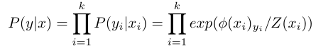
Here ϕ(.) is an activation function, k is a sequence length, and Z(xi) is a partition function. After that, P(y|x) can be written as follows:

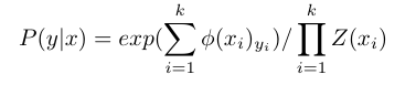
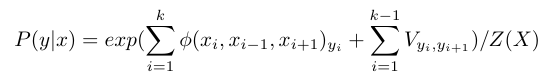
The above expression gives us an expression of P(y|x) when we use greedy decoding. In the case of Conditional Random Field, we need information about neighboring labels. This information is incorporated into the expression of P(y|x) with transition table V. In another variant of CRF, a context window on inputs x{i} is used to calculate along with labels information as well. For example, if there is a context window of 3, the expression for P(y|x) is given as follows:

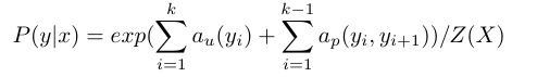
Let’s consider the following notation for both unary-log terms and pairwise transition terms, respectively.

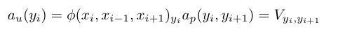
The expression of P(y|x) can be written as follows:

Inference

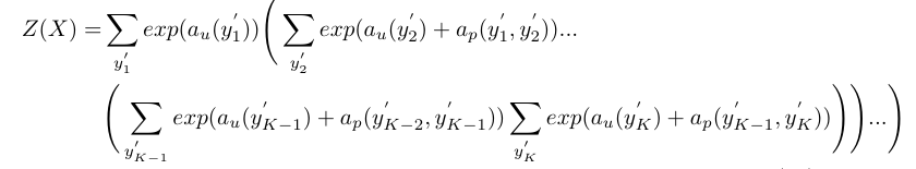
As we know, Z(X) is a partition function. If we calculate the partition function in a naively we obtain an expression for the partition function as follows:

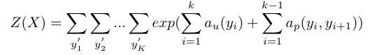
In the above expression, as we can see, we are doing K sums every time we calculate the partition function. The computational complexity for the above calculation is of the order O(C^K), which is not scalable. To reduce complexity, we need to arrange Z(X) in a slightly different way.

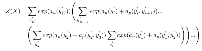
The advantage of such rearrangement of terms becomes visible in Algorithm 1 given below. We introduce another class of vector-valued functions α{i}(.), which is initialized by performing the innermost sum over all possible labels at y{1}’. Such rearrangement of terms allows us to leverage the advantages of dynamic programming to reduce the complexity of the task. A more detailed algorithm is given below.

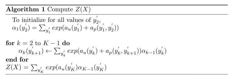
The computational complexity of the above algorithm is O(KC²), where C is the number of labels for each position.

Again, the sum for Z(X) is rearranged such that the innermost sum is performed over the Kth label of the sequence given and traversed from the Kth label to the first label of the sequence.

This time, we introduce another vector-valued function β(.). We initialize β function by summing over all possible labels at the Kth position and iterate till labels at 2nd position.

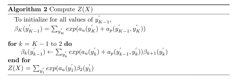
Computing the partition function from algorithm 1 (or 2) is referred to as the Forward-Backward algorithm for CRF. Computing α function is termed as a forward pass while computing β function is termed as a backward pass. The above processes together are also called belief propagation.

In this article, we first got an overview of graphical models. Then we discussed what is a conditional random field and its applications — its another variant based on the context. While making an inference, we saw the need for a forward-backward algorithm and its time complexity. Apart from these topics, we also should look into the loss function of CRF and how a back-propagation performed while training. These topics can be covered during another discussion.

References and Further Reading:

1. Youtube lecture series of Hugo Larochelle
2. http://www.cs.cmu.edu/~10715-f18/lectures/lecture2-crf.pdf
3. http://www.davidsbatista.net/blog/2017/11/13/Conditional_Random_Fields/
4. Conditional Random Fields: Probabilistic Models for Segmenting and Labeling Sequence Data (Paper)

---

A Tour of Conditional Random Field was originally published in Towards AI — Multidisciplinary Science Journal on Medium, where people are continuing the conversation by highlighting and responding to this story.

Published via Towards AI