Understanding Tree Models

Author(s): Nirmal Maheshwari

Originally published on Towards AI the World’s Leading AI and Technology News and Media Company. If you are building an AI-related product or service, we invite you to consider becoming an AI sponsor. At Towards AI, we help scale AI and technology startups. Let us help you unleash your technology to the masses.

Machine Learning

Life is full of decisions and eventually, we do measure which option to take on some logical-based analysis. In this series of blogs, we will be making ourselves comfortable with two extremely popular machine learning models — decision trees and random forests.

For this blog, we will limit ourselves to Decision trees and then move on to Random Forest one of the most used algorithms in the industry. We will also understand the coding part of the business by solving a real-world example. So let’s start.

The intuition behind Decision Tree

With high interpretability and an intuitive algorithm, decision trees mimic the human decision-making process and excel in dealing with categorical data. Unlike other algorithms such as logistic regression or SVMs, decision trees do not find a linear relationship between the independent and the target variable. Rather, they can be used to model highly nonlinear data.

This is a supervised learning algorithm and you can easily explain all the factors leading to a particular decision/prediction. Hence, they are easily understood by business people. Let us understand this with the below example of a Loan Approval System

We need to take a decision basis on this historical data if a new record comes in, whether that person is eligible for a loan or not. Let’s visualize the decision tree for the above dataset

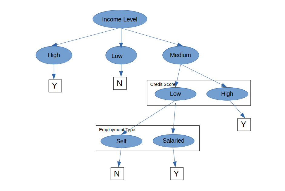
You can see that decision trees use a very natural decision-making process: asking a series of questions in a nested if-then-else structure.

On each node, you ask a question to further split the data held by the node. If the test passes, you go left; otherwise, you go right. We split at each node till we don’t get a pure subset or reach a decision.

Interpreting a Decision Tree

Let’s understand the above in terms of a decision tree.

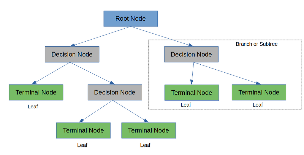
At every Decision Node, a test is conducted related to one of the features in the dataset and if the test is passed it goes to one side of the tree otherwise the other side. The outcome of the test will take us to one of the branches of the tree and for a classification problem each leaf will be containing one of the classes.

A binary decision tree is where we the test split the dataset into two parts like deciding on basis of employment type in the above example. Now if there is an attribute that has 4 kinds of values and depending on each value I want to make a decision then it will be a multiway decision tree.

The decision trees are easy to interpret. Almost always, you can identify the various factors that lead to the decision. Trees are often underestimated for their ability to relate the predictor variables to the predictions. As a rule of thumb, if interpretability by laymen is what you’re looking for in a model, decision trees should be at the top of your list.

Regression with Decision Trees

In regression problems, a decision tree splits the data into multiple subsets. The difference between decision tree classification and decision tree regression is that in regression, each leaf represents a linear regression model, as opposed to a class label. For this blog, we will keep ourselves limited to classification problems but I will mention certain points for regression as well wherever required.

Algorithms for Decision Tree Construction

Let us understand how does a decision tree knows on which attribute the split has to be taken first?

Concept of Homogeneity

In general, the rule says that we should try and split the nodes such that the resulting nodes are as homogenous as possible, i.e. all the rows belong to a single class after the split. If the node is income level in the above example, try and split it with a rule such that all the data points that pass the rule have one label (i.e. is as homogenous as possible), and those that don’t, have another.

Now from the above, we come to a general rule as below

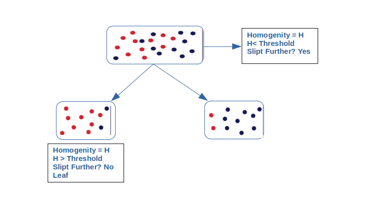
The rule says that we keep splitting the data till the homogeneity of the data is below a certain threshold, so you go step-by-step, picking an attribute and splitting the data such that the homogeneity increases after every split. You stop splitting when the resulting leaves are sufficiently homogenous. What is sufficiently homogenous? Well, you define the amount of homogeneity which, when achieved, the tree should stop splitting further. Let’s see what are some specific methods that are used to measure homogeneity.

Let us try to understand all the homogeneity measures with a hypothetical dataset example

We need to predict for a certain group of people depending on their age and gender, whether they will be able to play cricket or not.

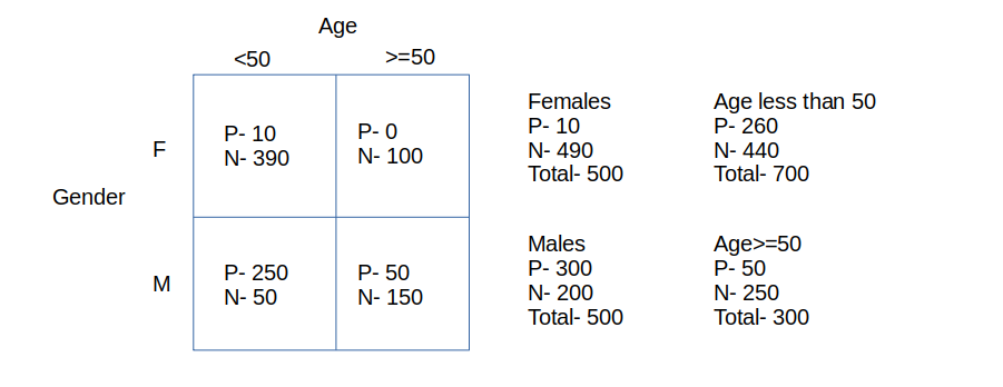
Now in the above example, we need to decide whether to split it on the age or gender to decide whether the person will be able to play cricket or not? Let’s look at the homogeneity measure to make the decision

Gini Index

Gini index uses the sum of the squares of the probabilities of various labels in the data set.

The total Gini index, if you split on gender, will be

Gini Index(gender) = (fraction of total observations in male-node)*Gini index of male-node + (fraction of total observations in female-node)*Gini index of female-node.

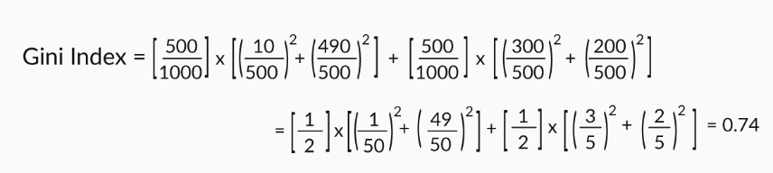
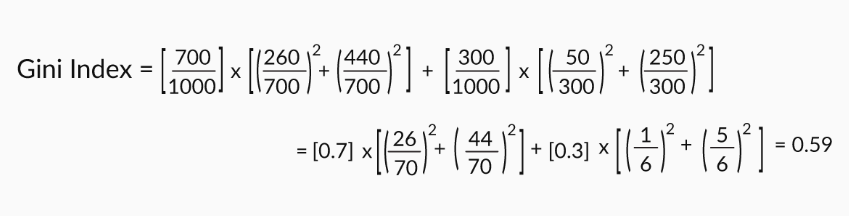
Similarly, we can calculate the Gini index if we split on age.

Assume that you have a data set with 2 class labels. If the data set is completely homogeneous (all the data points belong to label 1), then the probability of finding a data point corresponding to label 2 will be 0 and that of label 1 will be 1. So p1= 1, and p2= 0. The Gini index, equal to 1, will be the highest in such a case. The higher the homogeneity, the higher the Gini index.

So if you had to choose between two splits: age and gender. The Gini index of splitting on gender is higher than that of splitting on age; so you go ahead and split on gender.

Entropy and Information Gain

Another homogeneity measure is Information Gain. The idea is to use the notion of entropy. Entropy quantifies the degree of disorder in the data, and like the Gini index, its value also varies from 0 to 1.

Entropy is given by

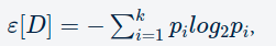
where p _i is the probability of finding a point with the label i, same as in Gini index and k is the number of different labels, and ε[D] is the entropy of the data set D.

Information Gain = ε[D]−ε[DA] i.e the entropy of the original dataset minus the weighted sum of the entropy of the partitions after you make a split.

Let’s consider an example. You have four data points out of which two belong to the class label ‘1’, and the other two belong to the class label ‘2’. You split the points such that the left partition has two data points belonging to label ‘1’, and the right partition has the other two data points that belong to label ‘2’. Now let’s assume that you split on some attribute called ‘A’.

1. Entropy of original/parent data set is ε[D]=−[(24)log2(24)+(24)log2(24)]=1.0.
2. The entropy of the partitions after splitting is ε[DA]=−0.5∗log2(2/2)−0.5∗log2(2/2)=0.
3. Information gain after splitting is Gain[D,A]=ε[D]−ε[DA]=1.0.

So, the information gain after splitting the original data set on attribute ‘A’ is 1.0, and the better the value of information gain, the better is the homogeneity of the data after the split.

For splitting done for continuous output variables? You calculate the Rsquare of data sets (before and after splitting) in a similar manner to what you do for linear regression models. So split the data such that the R2 of the partitions obtained after splitting is greater than that of the original or parent data set. In other words, the fit of the model should be as ‘good’ as possible after splitting.

I hope this blog will make you understand the Decision Trees in a very simple way. Next blog in the series we will be discussing the hyperparameters related to decision trees and also understand that “What is so random about Random Forest :)”

References

1. http://ogrisel.github.io/scikit-learn.org/sklearn-tutorial/modules/tree.html
2. https://www.udemy.com/course/complete-data-science-and-machine-learning-using-python/
3. Data Science Program by Upgrad(https://www.upgrad.com/)

Link to my medium profile

https://commondatascientist.medium.com/medium-to-bond-de3c81e193b8

---

Understanding Tree Models was originally published in Towards AI on Medium, where people are continuing the conversation by highlighting and responding to this story.

Join thousands of data leaders on the AI newsletter. It’s free, we don’t spam, and we never share your email address. Keep up to date with the latest work in AI. From research to projects and ideas. If you are building an AI startup, an AI-related product, or a service, we invite you to consider becoming a sponsor.

Published via Towards AI