Titanic Survival Prediction — II

Last Updated on January 6, 2023 by Editorial Team

Last Updated on March 5, 2021 by Editorial Team

Author(s): Hira Akram

Data Science

Titanic Survival Prediction — II

Predict who survived the sinking!

In the preceding article, we discussed the fundamental techniques of exploratory data analysis, data visualizations and pre-processing of raw data. We also established an understanding of the methods to engineer complex new features from original dataset. Moreover, common data preparatory practices like feature encoding and standard scaling were also covered.

In this article, let’s briefly discuss a number of algorithms that are extensively being used for binary classification along with their performance on the Titanic dataset. Moreover, we’ll train, test and evaluate our survival predictions based on different metrics.

How true is “Garbage In, Garbage Out’’?

While building a machine learning model doesn’t stress over which algorithm to pick, rather primarily focus on EDA and data mining because they play a very crucial role. There will be times when your model would constantly give the same performance despite plugging in different algorithms; instead of jumping from one algorithm to another, it is always advised to use the following practice:

1. Do some basic EDA using SQL, Excel or Python/R, however, preferred.
2. Impute the missing values.
3. Plot features that deem important and try to find underlying patterns.
4. Encode categorical features and normalize/standardize continuous ones.
5. Pick a simple algorithm and train the model straight away.
6. If you’re lucky, you might just get your desired output on the first go. In that case, rerun the model to validate your results.
7. In case you end up disappointed by the first run, observe how the model is behaving and whether you’ll need to collect more data or add new features etc.

Note: If you provide the right data to any algorithm, it is more likely that you will get your preferred outcome without having to go back-and-forth.

Binary Classifiers

Our aim was to identify passengers based on the given features like Age, SibSp, Pclass, Fare etc. who were more likely to have survived the ship wreck. For this binary classification problem let’s train five classifiers and compare their performances on the training dataset.

We’ll use the following supervised learning algorithms which can help us make survival predictions on the Titanic dataset:

• Random Forest Classifier
• Logistic Regression
• Gradient Boosting Classifier
• Support Vector Machine
• Naïve Bayes Classifier

Random Forest Classifier

Random Forest is a very flexible ensemble learning algorithm that can be used to solve both classification and regression problems using the bagging paradigm. The algorithm does random sampling with replacement and creates multiple copies of the dataset. As a result, a new prediction can be obtained by taking average of the sampling predictions for regression trees or by majority voting in case of a classification problem.

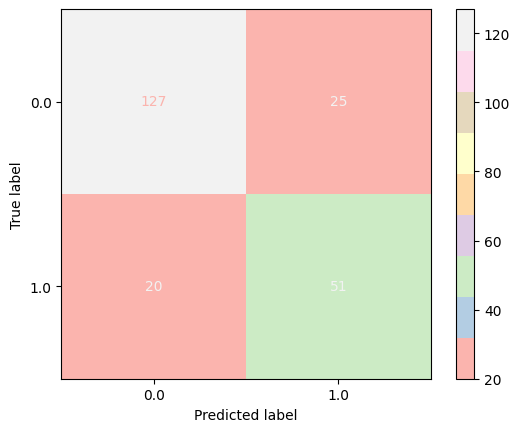
In our case, the overall performance of this model seemed pretty good on the training dataset. With a fair number of correct predictions, we were able to achieve satisfactory figures for both recall and f1 score. Illustrated below is the confusion matrix obtained from this classifier:

Logistic Regression

Logistic Regression belongs to the class of supervised learning algorithms. Contrary to what the name suggests, this algorithm is specifically used for making classification predictions. It aims to output two possible values based on which the class is defined. One such mathematical function which assigns values between our desired interval i.e. [0, 1] is called sigmoid. If this function returns a prediction closer to 0 we declare it as a negative class whereas, if the prediction lies closer to 1 it is considered to be positive and thus our targeted class.

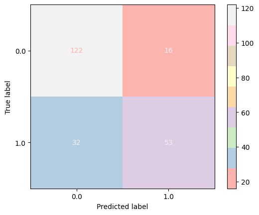
With this model we arrived at a somewhat similar result. However, the accuracy did show a slight decline. Having a higher number of true positives, our model’s precision significantly increased. Below figure shows the confusion matrix obtained from this model:

Gradient Boosting Classifier

Moving on to the next classifier which is an effective ensemble learning algorithm but unlike random forest this algorithm makes use of the boosting technique.

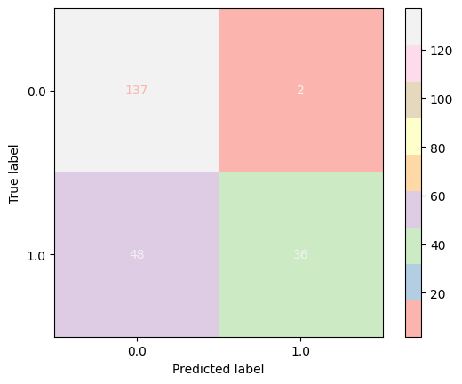
As it can be seen from the figure below that we correctly predicted a good number of true negatives and true positives and this model also outperformed in terms of precious. Moreover, it also gave a surprisingly low number of false positives:

Support Vector Machine

Due to it’s underlying mathematical principle support vector machine is also known as a Large Margin Classifier. There is a significant distance between the positive and negative examples separated by the decision boundary. As a result this decision boundary contributes towards better generalization of future examples.

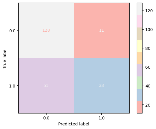
As the figure below shows that there is a huge number of falsely predicted labels and so this model failed to make acceptable predictions in our case:

Naïve Bayes Classifier

Lastly, we trained the data using Naïve Bayes classifier which is a super simple supervised learning algorithm. The underlying concept behind this classification technique is that is assumes that each feature statistically reflects the Bayes theorem i.e. each and every feature in a class is independent of one another.

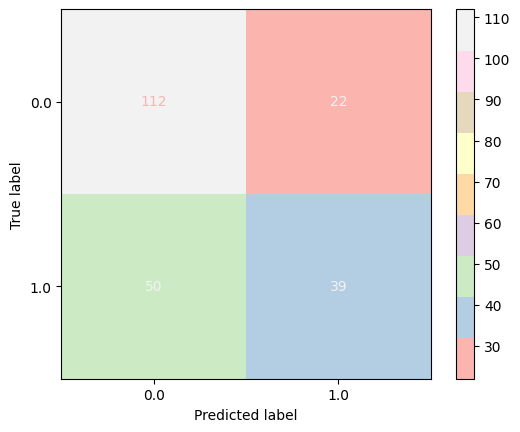
Based on the results drawn from this model we observed that it was not only unable to preserve accuracy but it was also particularly least efficient in terms of other metrics as well. Which is evident from the confusion matrix and Figure-1:

Performance Comparison

Typically, classifiers are evaluated on a wide range of metrics like Precision, Recall, F1-Score, Accuracy so on and so forth. These help us decide how well the model is behaving. Concretely, if we had only considered a single metric as our deciding factor, then we might have ended up with a different conclusion and there will always exist a trade-off.

Furthermore, its important to analyze the classifies through multiple deciding factors so that we are more confident about our selection. Earlier, we individually examined confusion matrix of each model to get an intuitive view about the correctly predicated labels. Now let’s also look into a few other factors to draw more accurate conclusions. As it can be seen in the figure below that we have taken into account accuracies of train and test dataset, precision, recall and f1-score of each model. These results however, show that the accuracy figures are relatively acceptable in each scenario but when other factors are brought under consideration then clearly ‘Random Forest Classifier’ outperformed all in all.

Figure below shows a complete comparison between all five models that we’ve trained so far:

Conclusion

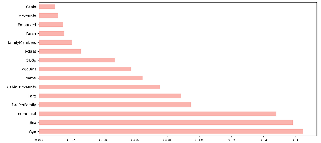
Now that we have finalized our model selection, let’s move forward with the testing phase. Random forest also provides us with an option to limit ourselves to features which add significant value towards determining the data trend. Below is a list of important features:

features = pd.Series(rfc.feature_importances_, index=X_train.columns).sort_values()

features.plot(kind='barh', cmap='Pastel1')

Let’s only utilize the ones that have value ≥ 0.06 so that we retrain our model based on features that have a higher impact in searching for hidden patterns within our dataset. Here’s a link to the GitHub project for reference.

Thanks for reading! ^_^

---

Titanic Survival Prediction — II was originally published in Towards AI on Medium, where people are continuing the conversation by highlighting and responding to this story.

Published via Towards AI