The Art and Science of Regularization in Machine Learning: A Comprehensive Guide

Author(s): Data Science meets Cyber Security

Originally published on Towards AI the World’s Leading AI and Technology News and Media Company. If you are building an AI-related product or service, we invite you to consider becoming an AI sponsor. At Towards AI, we help scale AI and technology startups. Let us help you unleash your technology to the masses.

REGULARIZATION IN MACHINE LEARNING: A PRACTICAL GUIDE

INTRODUCTION:

Are you tired of your machine learning models performing poorly on new data? Are you sick of seeing your model’s validation accuracy skyrocket only to crash and burn on the test set? If so, it’s time to learn about regularisation!

Regularisation is a technique that is used to prevent overfitting in machine learning models.

LET’S GET OUR BASICS CLEAR FIRST :

We’ll go through some interesting analogies and practical implementation of concepts to get things crystal clear in our heads.

OVERFITTING :

Overfitting occurs when a model is too complex and fits the training data too well, but is not able to generalise well to new, unseen data. This can lead to poor performance on the test set or in real-world applications.

LET’S UNDERSTAND IT WITH MORE BETTER ANALOGY:

Imagine a child who has learned to recognize dogs by seeing pictures of only golden retrievers. When shown a picture of a different dog breed, such as a poodle, the child is unable to recognize it as a dog because they have only learned to recognize a specific type of dog rather than having a general understanding of what features define a dog. This is similar to how a model can overfit the training data and be unable to generalize well to new, unseen data.

LET’S LOOK THROUGH IT PRACTICALLY:

import numpy as np
import matplotlib.pyplot as plt
 
# Generate data
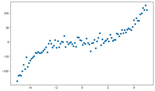
x = np.linspace(-5, 5, 100)
y = x**3 + np.random.normal(0, 10, 100)
 
# Create figure with larger size
fig, ax = plt.subplots(figsize=(10, 6))
 
# Plot data
ax.plot(x, y, 'o')
plt.show()

This generates a set of 100 x-values and corresponding y-values, with the y-values being a cubic function of the x-values with some added noise. The data is plotted as follows:

Next, we can fit a polynomial regression model to the data:

from sklearn.linear_model import LinearRegression
from sklearn.preprocessing import PolynomialFeatures
 
# Create polynomial features
poly = PolynomialFeatures(degree=10)
x_poly = poly.fit_transform(x.reshape(-1, 1))
 
# Fit model to data
model = LinearRegression()
model.fit(x_poly, y)
 
# Predict on original x values
y_pred = model.predict(x_poly)
 
# Create figure and plot data
fig, ax = plt.subplots(figsize=(10, 6))
ax.plot(x, y, 'o', label='True data')
ax.plot(x, y_pred, 'o', label='Predicted data')
ax.legend()
 
# Display figure
plt.show()

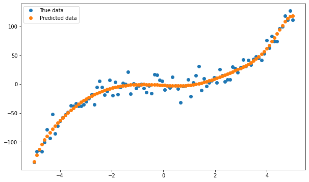
This fits a polynomial regression model with a degree of 10 to the data, which is a very high degree and results in a very complex model. The model has plotted along with the original data as follows:

CONCLUSION:

We can see that the model is able to fit the training data very well but is not able to generalize well to new, unseen data. This is an example of overfitting, as the model has learned the specific patterns in the training data but has not developed a general understanding of the underlying relationships in the data.

To prevent overfitting, we can use techniques such as regularisation or early stopping to reduce the complexity of the model and improve its generalization performance.

UNDERFITTING:

Under-fitting, on the other hand, occurs when a model is too simple and is unable to capture the underlying patterns in the data. This can also lead to poor performance, but for a different reason.

LET’S UNDERSTAND IT WITH MORE BETTER ANALOGY:

One way to understand underfitting is through the analogy of a student preparing for a test. Imagine that a student is studying for a history test and is given a textbook to read. However, the student only reads the first few pages of the textbook and does not fully grasp the material. On the day of the test, the student is unable to answer even the most basic questions because they have not learned enough about the subject.

This is similar to how a model can underfit the training data. The model is too simple and is unable to capture the underlying patterns in the data, leading to poor performance on the training set and poor generalization to new, unseen data.

On the other hand, if the student had taken the time to read and fully understand the entire textbook, they would have been better equipped to perform well on the test. Similarly, a model that has not underfitted to the training data and has a good generalization performance will be able to make accurate predictions on the training data and new, unseen data.

Here is a simple code example that demonstrates underfitting using a linear regression model:

import numpy as np
import matplotlib.pyplot as plt
from sklearn.linear_model import LinearRegression
 
# Generate synthetic data
x = np.linspace(-5, 5, 50)
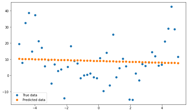
y = x**2 + np.random.normal(0, 10, 50)
 
# Fit linear model
model = LinearRegression()
model.fit(x.reshape(-1, 1), y)
 
# Predict on training data
y_pred = model.predict(x.reshape(-1, 1))
 
# Create figure with specified size
plt.figure(figsize=(10, 6))
 
# Plot data and predictions
plt.plot(x, y, 'o', label='True data')
plt.plot(x, y_pred, 'o', label='Predicted data')
plt.legend()
 
# Save figure to file
plt.savefig('figure.png', bbox_inches='tight')
 
# Show plot
plt.show()

CONCLUSION :

In this example, we generate synthetic data that follows a quadratic trend and fit a linear model to the data. We can see that the linear model is unable to capture the underlying quadratic trend and is under-fitting to the data, resulting in poor performance on the training set.

“Feeling lost when it comes to the connection between bias, variance, under-fitting, and overfitting? Don’t worry, I’ve got the answers you need!”

BIAS, VARIANCE, AND ITS CONNECTION TO OVERFITTING AND UNDERFITTING:

BIAS and VARIANCE are two important concepts that describe the error of a machine learning model. Bias refers to the error due to incorrect assumptions in the model, while variance refers to the error due to the complexity of the model.

In general, we want to find a model that has low bias and low variance, as this will result in good generalization performance on the test set or in real-world applications. However, it is often not possible to simultaneously minimize both bias and variance, and we must find a balance between the two.

UNDERFITTING occurs when a model is too simple and is unable to capture the underlying patterns in the data, leading to high bias and low variance.

OVERFITTING occurs when a model is too complex and fits the training data too well but is not able to generalize well to new, unseen data, leading to low bias and high variance.

LET’S UNDERSTAND THROUGH AN EXAMPLE:

Consider a model that is trying to predict the price of a house based on its size and location. If the model is too simple and only uses the size of the house as a feature, it may have high bias and low variance. This model may make consistent but inaccurate predictions because it is unable to capture the influence of the location on the price. On the other hand, if the model is too complex and uses many features that are not relevant to the price of the house, it may have low bias and high variance. This model may make accurate predictions on the training data but may not generalize well to new, unseen data.

Therefore, it is important to find a model that strikes a balance between bias and variance and has good generalization performance. Regularisation is one way to control the bias-variance trade-off and find this balance.

MATHS BEHIND THIS? (BECAUSE EVERYTHING IS CONNECTED TO MATHS, AFTER ALL: )

BIAS:

The bias of a model is the difference between the expected prediction of the model and the true value. Mathematically, it can be written as:

BIAS = E[F(X)] — F(X)

where f(x) is the true value, and E[f(x)] is the expected prediction of the model.

VARIANCE:

The variance of a model is the variability of the model’s predictions for a given input. Mathematically, it can be written as:

VARIANCE = E[(F(X) — E[F(X)])²]

where f(x) is the prediction of the model for a given input x and E[f(x)] is the expected prediction of the model.

Code example that demonstrates how bias and variance are related to overfitting and underfitting in a linear regression model:

import numpy as np
import matplotlib.pyplot as plt
from sklearn.linear_model import LinearRegression
from sklearn.model_selection import train_test_split
 
# Generate synthetic data
x = np.linspace(-5, 5, 50)
y = x**2 + np.random.normal(0, 10, 50)
 
# Split data into training and test sets
x_train, x_test, y_train, y_test = train_test_split(x, y, test_size=0.2)
 
# Fit linear model to training data
model = LinearRegression()
model.fit(x_train.reshape(-1, 1), y_train)
 
# Predict on training and test sets
y_train_pred = model.predict(x_train.reshape(-1, 1))
y_test_pred = model.predict(x_test.reshape(-1, 1))
 
# Create figure with specified size
plt.figure(figsize=(10, 6))
 
# Plot data and predictions
plt.plot(x, y, 'o', label='True data')
plt.plot(x_train, y_train_pred, 'o', label='Predictions on training set')
plt.plot(x_test, y_test_pred, 'o', label='Predictions on test set')
plt.legend()
plt.show()

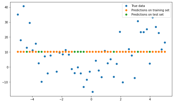
CONCLUSION:

We generate synthetic data that follows a quadratic trend, and split the data into a training set and a test set. We then fit a linear model to the training set and make predictions on both the training set and the test set.

We can see that the model has a low bias on the training set, as it is able to fit the data well. However, the model has high variance on the test set, as it is not able to generalize well to new, unseen data. This demonstrates how bias and variance are related to overfitting and underfitting in a linear regression model.

SO HOW DO WE STRIKE A BALANCE BETWEEN OVERFITTING AND UNDERFITTING?

ENTER REGULARISATION!

Regularisation is a method that adds a penalty term to the objective function that the model is trying to optimize. This penalty term helps to reduce the complexity of the model by encouraging the model to use only the most important features and reducing the influence of less important ones.

There are several different types of regularisation techniques, but the three most commonly used are Ridge, Lasso, and Elastic Net.

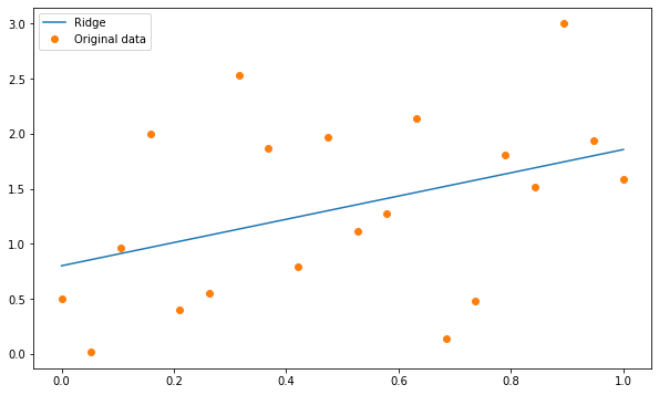
RIDGE REGULARISATION:

Ridge regularisation, also known as L2 regularisation, adds a penalty term to the objective function that is proportional to the square of the model weights. This results in a model with more uniformly distributed weights, which can help to prevent overfitting.

CODE — IMPLEMENTATION:

import numpy as np
import matplotlib.pyplot as plt
from sklearn.linear_model import Ridge, Lasso, ElasticNet
from sklearn.preprocessing import StandardScaler

# Generate synthetic data
np.random.seed(42)
m = 20
X = np.linspace(0, 1, m).reshape(-1, 1)
y = 3 * X + np.random.randn(m, 1)
 
# Scale the data
scaler = StandardScaler()
X_scaled = scaler.fit_transform(X)
 
# Create the model
ridge = Ridge(alpha=1.0)
 
# Fit the model
ridge.fit(X_scaled, y)
 
# Predict using the model
y_pred_ridge = ridge.predict(X_scaled)
 
# Create figure with specified size
plt.figure(figsize=(10, 6))
 
# Plot the predictions
plt.plot(X, y_pred_ridge, label='Ridge')
plt.plot(X, y, 'o', label='Original data')
plt.legend()
plt.show()

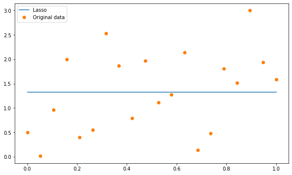
LASSO REGULARISATION:

Lasso regularisation, also known as L1 regularisation, adds a penalty term to the objective function that is proportional to the absolute value of the model weights. This results in a model with fewer non-zero coefficients, which can be useful for feature selection.

CODE — IMPLEMENTATION:

# Generate synthetic data
np.random.seed(42)
m = 20
X = np.linspace(0, 1, m).reshape(-1, 1)
y = 3 * X + np.random.randn(m, 1)
 
# Scale the data
scaler = StandardScaler()
X_scaled = scaler.fit_transform(X)
 
# Create the model
lasso = Lasso(alpha=1.0)
 
# Fit the model
lasso.fit(X_scaled, y)
 
# Predict using the model
y_pred_lasso = lasso.predict(X_scaled)
 
# Create figure with specified size
plt.figure(figsize=(10, 6))
 
# Plot the predictions
plt.plot(X, y_pred_lasso, label='Lasso')
plt.plot(X, y, 'o', label='Original data')
plt.legend()
plt.show()

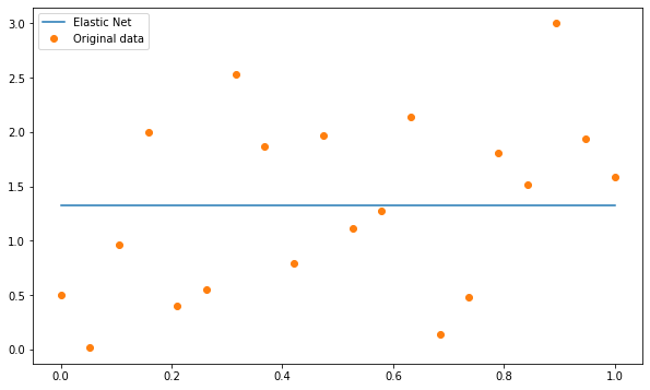
ELASTIC NET REGULARISATION:

It is a combination of Ridge and Lasso regularisation, and it allows for a balance between the two.

So how do we use these regularisation techniques in practice? Let’s take a look at an example using simulated data.

CODE — IMPLEMENTATION:

# Generate synthetic data
np.random.seed(42)
m = 20
X = np.linspace(0, 1, m).reshape(-1, 1)
y = 3 * X + np.random.randn(m, 1)
 
# Scale the data
scaler = StandardScaler()
X_scaled = scaler.fit_transform(X)
 
# Create the model
elastic_net = ElasticNet(alpha=1.0, l1_ratio=0.5)
 
# Fit the model
elastic_net.fit(X_scaled, y)
 
# Predict using the model
y_pred_elastic_net = elastic_net.predict(X_scaled)

# Create figure with specified size
plt.figure(figsize=(10, 6))
 
# Plot the predictions
plt.plot(X, y_pred_elastic_net, label='Elastic Net')
plt.plot(X, y, 'o', label='Original data')
plt.legend()
plt.show()

SUMMING UP THE BLOG BY THINGS TO KEEP IN MIND:

1. Regularisation is a technique used to improve the generalization of a model by preventing it from overfitting the training data.
2. Ridge, lasso, and elastic net are all types of regularisation that can be applied to linear regression models.
3. Ridge regularisation adds a penalty term that is the sum of the squares of the model coefficients, while lasso regularisation adds a penalty term that is the sum of the absolute values of the model coefficients. Elastic net regularisation is a combination of the two.
4. The strength of the regularisation is controlled by a hyper-parameter, which should be chosen carefully using cross-validation.
5. Ridge, lasso, and elastic net regularisation can all be used to select relevant features in a dataset by driving some of the model coefficients to exactly zero.
6. It is often useful to try multiple regularisation methods and compare their performance to choose the most appropriate one for a given problem.
7. Regularisation is not always necessary, and in some cases, a simple linear model may perform just as well as a regularised model.

ONE MYTH VS FACT (BECAUSE WHY NOT!):

MYTH:

Ridge, lasso, and elastic net regularisation can be used interchangeably for any problem.

FACT:

Each type of regularisation has unique properties and may be more or less suitable for a given problem. Ridge is best for datasets with many features, the lasso is good for feature selection, and the elastic net is a combination of the two that may work well for datasets with many features and some correlated features. It is best to try multiple methods and compare their performance.

STAY TUNED FOR THE NEXT BLOG WHERE WE’LL TRY TO BUILD THE

“ REGULARISATION MODEL FOR INTRUSION DETECTION ” 🤯

FOLLOW US FOR THE SAME FUN TO LEARN DATA SCIENCE BLOGS AND ARTICLES: 💙

LINKEDIN: https://www.linkedin.com/company/dsmcs/

INSTAGRAM: https://www.instagram.com/datasciencemeetscybersecurity/?hl=en

GITHUB: https://github.com/Vidhi1290

TWITTER: https://twitter.com/VidhiWaghela

MEDIUM: https://medium.com/@datasciencemeetscybersecurity-

WEBSITE: https://www.datasciencemeetscybersecurity.com/

---

The Art and Science of Regularization in Machine Learning: A Comprehensive Guide was originally published in Towards AI on Medium, where people are continuing the conversation by highlighting and responding to this story.

Join thousands of data leaders on the AI newsletter. It’s free, we don’t spam, and we never share your email address. Keep up to date with the latest work in AI. From research to projects and ideas. If you are building an AI startup, an AI-related product, or a service, we invite you to consider becoming a sponsor.

Published via Towards AI