Text Similarity using K-Shingling, Minhashing and LSH(Locality Sensitive Hashing)

Last Updated on October 29, 2021 by Editorial Team

Author(s): Supriya Ghosh

Natural Language Processing

Text Similarity using K-Shingling, Minhashing, and LSH(Locality Sensitive Hashing)

Text similarity plays an important role in Natural Language Processing (NLP) and there are several areas where this has been utilized extensively. Some of the applications include Information retrieval, text categorization, topic detection, machine translation, text summarization, document clustering, plagiarism detection, news recommendation, etc. encompassing almost all domains.

But sometimes, it becomes difficult to understand the concept behind the Text Similarity Algorithms. This write-up will show an implementation of Text Similarity along with an explanation of the required concepts.

But before I start, let me tell you that there might be several ways and several algorithms to perform the same task. I will use one of the ways for depiction using K-Shingling, Minhashing, and LSH(Locality Sensitive Hashing).

Dataset considered is Text Extract from 3 documents for the problem at hand.

We can use n — number of documents with each document being of significant length. But to make it simpler and avoid heavy computations, I am considering a small chunk from each document.

Let’s perform the implementation in Steps.

Step 1 :

Set your working directory to the folder where the files are placed so that R can read it. Then read all the input files from the working directory using the below code.

# Libraries used
library(dplyr)
library(proxy)
library(stringr)
library(data.table)
# Set the working directory
setwd(".\")

# Read the original text file 
files <- list.files(path=".", pattern='*.txt', all.files=FALSE,
           full.names=FALSE)

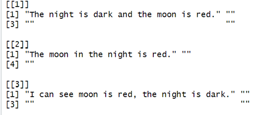
( doc <- lapply( files, readLines ) )

R Studio Input Display

Step 2 :

Preprocess the text to remove punctuation, convert it into lower cases, and split text into word by word.

# Preprocess text
documents <- lapply(doc, function(x) {
  text <- gsub("[[:punct:]]", "", x) %>% tolower()
  text <- gsub("\\s+", " ", text) %>% str_trim()  
  word <- strsplit(text, " ") %>% unlist()
  return(word)
})
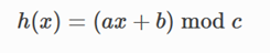
# Print the texts in files
documents[[1]]
documents[[2]]
documents[[3]]

R Studio Display

Step 3 :

Introduce K-Shingling which is a technique of representing documents assets. We will understand further the importance of K-Shingling but as of now, we can just try getting familiar with the Steps.

K-shingle of a document at hand is said to be all the possible consecutive sub-string of length k found in it.

Let’s illustrate with an example with k = 3.

Shingling <- function(document, k) {
  shingles <- character( length = length(document) - k + 1 )
  
  for( i in 1:( length(document) - k + 1 ) ) {
    shingles[i] <- paste( document[ i:(i + k - 1) ], collapse = " " )
  }
  
  return( unique(shingles) )  
}

# "shingle" the example document, with k = 3
documents <- lapply(documents, function(x) {
  Shingling(x, k = 3)
})
list( Original = doc[[1]], Shingled = documents[[1]] )

R Studio Display

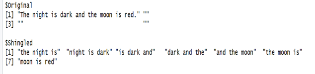
Hence with k = 3, the k-shingles of the first document which got printed out, consist of sub-strings of length 3.

The first K-Shingle is: “the night is”

The second Shingle is: “night is dark” and so on.

One important point to note is that a document’s k-shingle set should be unique. For example, if the first document above contains more than one “the night is” then it will only appear once as the set of k-shingle for that document.

Step 4:

Construct a “Characteristic” matrix that visualizes the relationships between the three documents. The “characteristic” matrix will be a Boolean matrix, with :

rows = the elements of every unique possible combination of shingles set across all documents.

columns = one column per document.

Thus, the matrix will be filled with 1 in row i and column j if and only if document j contains the shingle i , otherwise it will be filled with 0.

Let us try to understand this with the below depiction.

# Unique shingles sets across all documents
doc_dict <- unlist(documents) %>% unique()

# "Characteristic" matrix
Char_Mat <- lapply(documents, function(set, dict) {
  as.integer(dict %in% set)
}, dict = doc_dict) %>% data.frame()

# set the names for both rows and columns
setnames( Char_Mat, paste( "doc", 1:length(documents), sep = "_" ) )
rownames(Char_Mat) <- doc_dict
Char_Mat

R Studio Display

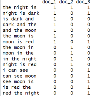
The first row of the above matrix has all three columns as 1. This is because all three documents contain the 3-shingle “the night is”.

For the second column, the value is [1, 0, 1] which means that document 2 does not have the 3-shingle “night is dark, while document 1 and 3 has.

One important point noted here is that most of the time these “characteristic matrices” are almost sparse. Therefore, we usually try to represent these matrices only by the positions in which 1 appears, so as to be more space-efficient.

Step 5 :

After creating shingle sets and characteristic matrix, we now need to measure the similarity between documents.

We will make use of Jaccard Similarity for this purpose.

For example, with two shingle sets as set1 and set2, the Jaccard Similarity will be :

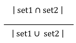
With this we will calculate the pairwise Jaccard similarities for all three documents. “dist” function in “R” quickly computes and returns the distance/similarity matrix.

# how similar is two given document, Jaccard similarity 
JaccardSimilarity <- function(x, y) {
  non_zero <- which(x | y)
  set_intersect <- sum( x[non_zero] & y[non_zero] )
  set_union <- length(non_zero)
  return(set_intersect / set_union)
}

# create a new entry in the registry
pr_DB$set_entry( FUN = JaccardSimilarity, names = c("JaccardSimilarity") )

# Jaccard similarity distance matrix 
d1 <- dist( t(Char_Mat), method = "JaccardSimilarity" )

# delete the new entry
pr_DB$delete_entry("JaccardSimilarity")
d1

doc

R Studio Display

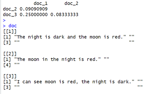
The similarity matrix d1 tells us that document 1 and 3 is the most similar among the three documents.

For small datasets, the above method works perfectly fine, but imagine if we have a large number of documents to compare instead of just three that too with significantly larger lengths, then the above method might not scale well, and we might have heavy computation with performance issue building up as the sparse matrices with a set of unique shingles across all documents will be fairly large, making computation of the Jaccard similarity between the documents a burden.

Under such situations, we employ a different technique that help us save computations and can compare document similarities on a large scale efficiently. The technique is called Minhashing.

Step 6 :

Minhashing involves compressing the large sets of unique shingles into a much smaller representation called “signatures”.

We then use these signatures to measure the similarity between documents.

Although it is impossible for these signatures to give the exact similarity measure, the estimates are pretty close.

The larger the number of signatures chosen, the more accurate the estimate is.

For illustration let us consider an example.

Suppose we take up the above example to minhash characteristic matrix of 16 rows into 4 signatures. Then the first step is to generate 4 columns of randomly permutated rows that are independent of each other. We can see for ourselves that this simple hash function does in fact generate random permutated rows. To generate this, we use the formula:

Where :

x is the row numbers of your original characteristic matrix.

a and b are any random numbers smaller or equivalent to the maximum number of x, and they both must be unique in each signature.

For e.g. For signature 1, if 5 is generated to serve as a- coefficient, it must be ensured that this value does not serve as a- coefficient multiple times within signature 1, though it can still be used as

b- coefficient in signature 1. And this restriction refreshes for the next signature as well, that is, 5 can be used to serve as a or b coefficient for signature 2, but again no multiple 5 for signature 2’s a or b coefficient and so on.

c is a prime number slightly larger than the total number of shingle sets.

For the above example set, since the total row count is 16, thus prime number 17 will do fine.

Now let’s generate this through the “R” code.

# number of hash functions (signature number)
signature_num <- 4

# prime number
prime <- 17

# generate the unique coefficients  
set.seed(12345)
coeff_a <- sample( nrow(Char_Mat), signature_num )
coeff_b <- sample( nrow(Char_Mat), signature_num )

# see if the hash function does generate permutations
permute <- lapply(1:signature_num, function(s) {
  hash <- numeric( length = length(nrow(Char_Mat)) )
  for( i in 1:nrow(Char_Mat) ) {
    hash[i] <- ( coeff_a[s] * i + coeff_b[s] ) %% prime
  }
  return(hash)
})
# # convert to data frame 
permute_df <- structure( permute, names = paste0( "hash_", 1:length(permute) ) ) %>%
  data.frame()
permute_df

R Studio Display

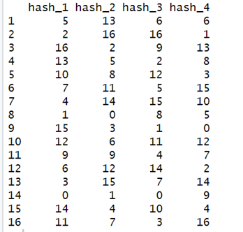
From the above output, we see that the 4 columns of randomly permutated rows got generated. There are 0s also, but it will not affect our computation and we will see this later.

Step 7 :

Using the randomly permutated rows, now signatures will be calculated further. The signature value of any column (document) is obtained by using the permutated order generated by each hash function, the number of the first row in which the column has a 1.

What we will do further is combine randomly permutated rows (generated by hash functions) with the original characteristic matrix and change the row names of the matrix to its row number to illustrate the calculation.

# use the first two signature as an example
# bind with the original characteristic matrix
Char_Mat1 <- cbind( Char_Mat, permute_df[1:2] )
rownames(Char_Mat1) <- 1:nrow(Char_Mat1)
Char_Mat1

R Studio Display

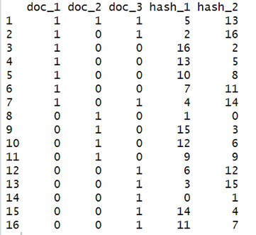
Now considering the matrix generated above, we will start with the first hash function (hash_1).

According to our first hash function’s permutated row order, the first row is row 14 ( why row 14 ? because 0 is the smallest value for our randomly generated permutation, and it has a 0 in row 14, making it the first row ). Then we’ll look at row 14’s entry for all three documents and try to find “which document’s entry at row 14 is a 1 ?”. document 3’s (doc_3) row 14 is a 1, thus the signature value for document 3 generated by our first hash function is 0. But documents 2 and 3’s entries at row 14 are both 0, thus we’ll have to continue looking.

According to our first hash function’s permutated row order, the second row is row 8 ( 1 is the second smallest value for our randomly generated permutation, and it has a value of 1 at row 8 ). We apply the same concept as above and find that document 2’s (doc_2) entry for row 8 is a 1, thus the signature value for document 2 generated by our first hash function is 1. Note that we’re already done with document 3, we do not need to check if it contains a 1 anymore. But we’re still not done, document 1’s entry at row 8 is still a 0. Hence, we’ll have to look further.

Again, checking the permutated row order for our first hash function, the third row is row 2. document 1’s entry for row 2 is 1. Therefore, we’re done with calculating the signature values for all three columns using our first hash function!! Which are [2, 1, 0].

We can then apply the same notion to calculate the signature value for each column (document) using the second hash function, and so on for the third, fourth, etc. A quick look at the signature second hash function shows that the first row according to its permutated row order is row 8 and doc_2 has a 1 in row 3. Similarly, the second row is row 14 with doc_3 as 1 and the third row is row3 with doc_1 as 1. Hence, the signature values generated by our second hash function for all three documents are [2, 0, 1].

As for these calculated signature values, we will store them into a signature matrix along the way, which will later replace the original characteristic matrix. The following section will calculate the signature values for all 3 columns using all 4 hash functions and print out the signature matrix.

# obtain the non zero rows' index for all columns
non_zero_rows <- lapply(1:ncol(Char_Mat), function(j) {
  return( which( Char_Mat[, j] != 0 ) )
})

# initialize signature matrix
SM <- matrix( data = NA, nrow = signature_num, ncol = ncol(Char_Mat) )

# for each column (document)
for( i in 1:ncol(Char_Mat) ) {
  # for each hash function (signature)'s value 
  for( s in 1:signature_num ) {
    SM[ s, i ] <- min( permute_df[, s][ non_zero_rows[[i]] ] )
  }
}

# set names for clarity
colnames(SM) <- paste( "doc", 1:length(doc), sep = "_" )
rownames(SM) <- paste( "minhash", 1:signature_num, sep = "_" )  
SM

R Studio Display

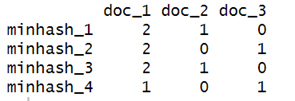
Our signature matrix has the same number of columns as the original characteristic matrix, but it only has n rows, where n is the number of hash functions we wish to generate (in this case 4).

Let me elaborate on how do we interpret the above result?

For e.g., for documents 1 and 3 (columns 1 and 3), its similarity would be 0.25 because they only agree in 1 row out of a total of 4 (both columns’ row 4 is 1).

Let’s calculate the same explanation through code.

# signature similarity
SigSimilarity <- function(x, y) mean( x == y )

# same trick to calculate the pairwise similarity 
pr_DB$set_entry( FUN = SigSimilarity, names = c("SigSimilarity") )
d2 <- dist( t(SM), method = "SigSimilarity" )
pr_DB$delete_entry("SigSimilarity")

list(SigSimilarity = d2, JaccardSimilarity = d1)

R Studio Display

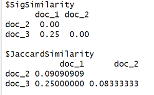
From the difference of the result between the original Jaccard similarity and the new similarity obtained using the signature similarity, we might doubt if this is an accurate estimate? But as mentioned earlier, Minhash's purpose is to provide a fast “approximation” to the true Jaccard similarity and the estimate can be closer but not 100% accurate hence the difference. Also, the example considered here is way too small to depict closer accuracy using the law of large numbers. More accurate and close results are expected with large datasets.

In cases where the primary requirement is to compute the similarity of every possible pair, probably for text clustering or so, then LSH (Locality Sensitive Hashing) does not serve the purpose but if the requirement is to find the pairs that are most likely to be similar, then a technique called Locality Sensitive Hashing can be employed further which I am discussing below.

Locality Sensitive Hashing

While the information necessary to compute the similarity between documents has been compressed from the original sparse characteristic matrix into a much smaller signature matrix, but the underlying problem or need to perform pairwise comparisons on all the documents still exists.

The concept for locality-sensitive hashing (LSH) is that given the signature matrix of size n (row count), we will partition it into b bands, resulting in each band with r rows. This is equivalent to the simple math formula — n = br, thus when we are doing the partition, we have to be sure that the b we choose is divisible by n. Using the signature matrix above and choosing the band size to be 2 the above example will become :

# number of bands and rows
bands <- 2
rows <- nrow(SM) / bands

data.frame(SM) %>% 
  mutate( band = rep( 1:bands, each = rows ) ) %>%
  select( band, everything() )

R Studio Display

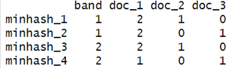
What locality-sensitive hashing tells us is: If the signature values of two documents agree in all the rows of at least one band, then these two documents are likely to be similar and should be compared (list it as the candidate pair). Using this small set of documents might be a bad example since it can happen that none of them will get chosen as our candidate pair. For instance, if the signature value of document 2 for band 1 becomes [ 0, 1 ] instead of the current [ 1, 0 ], then document 2 and document 3 will become a candidate pair as both of their rows in band1 takes the same value of [ 0, 1 ].

Note — My computations and your computations, while executing the above set of R Codes might vary as the signatures are randomly generated.

Final Thoughts

The above technique using Jaccard Similarity, Minhashing, and LSH is one of the utilized techniques to compute document similarity although many more exists. Text similarity is an active research field, and techniques are continuously evolving. Hence which method to use is very much dependent on the Use Case and the requirements of what we want to achieve.

Thanks for reading !!!

You can follow me on medium as well as

LinkedIn: Supriya Ghosh

Twitter: @isupriyaghosh

---

Text Similarity using K-Shingling, Minhashing and LSH(Locality Sensitive Hashing) was originally published in Towards AI on Medium, where people are continuing the conversation by highlighting and responding to this story.

Published via Towards AI