Survival Analysis: Produce a Single Time-to-Event Prediction from Survival Functions

Author(s): Yael Vilk

Originally published on Towards AI the World’s Leading AI and Technology News and Media Company. If you are building an AI-related product or service, we invite you to consider becoming an AI sponsor. At Towards AI, we help scale AI and technology startups. Let us help you unleash your technology to the masses.

Survival analysis is a family of statistical methods for analyzing time-to-event data. Traditionally, this technique was used in the health and insurance domains, where the event of interest would be death, re-hospitalization, and similarly morbid events. However, survival analysis can be applied to model any time period, like the time it takes for a person to get a job, a system to fail, or a customer to churn.

Survival analysis is unique in its ability to handle censored data, that is, data where the time-to-event information is not fully disclosed for some of the subjects. This can happen for different reasons. For example, it is possible a subject dropped out of the study before its termination or that the trial ended before the event of interest occurred for some of the subjects.

Applying different survival analysis techniques results in a single or multiple survival function. A survival function describes the probability of a subject, or a group, to survive past time T. In this context, ‘survival’ means avoiding the event of interest. The overall survival time, or lifespan, is the period of time between the ‘birth’ – trial onset, and ‘death’ – when the event of interest occurs. Naturally, the function is monotonically non-increasing, as survival only becomes less likely with time.

Here’s a survival function, for example:

import pandas as pd

pd.DataFrame({'t': [1, 2, 5, 7, 9, 10, 12, 13], 'S(t)': [98, 95, 90, 80, 60, 50, 40, 0]}).set_index('t')

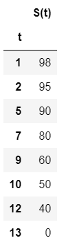
According to this survival function, there is a 90% chance that the event of interest will not occur by time 5.

Survival functions are also useful for comparing survival times of several groups and for describing the effect of additional variables on survival time. It is a powerful function that holds a lot of information, but sometimes, you want to summarize it into a single time-to-event prediction. In this post, I will discuss the multiple ways to predict a lifespan from a survival function. If you wish to learn more about survival analysis in general or how to actually obtain a survival function(s) from your data, try the documentation of the python library ‘lifelines’, or this great blog post.

Let’s get some survival functions.

We’ll start by creating a toy dataset in python. In this dataset, we have 5 subjects in a study that lasted over 20 days. The “observed” column states whether the subjects have indeed experienced the recurrence of the symptoms during the study, and the “duration” column denotes the day on which the symptoms reappeared. As you can see, our data is not censored: the time of symptom recurrence was recorded for the entire sample. We have also documented a predictor variable.

df = pd.DataFrame({"predictor": [5, 3.5, 20, 9, 15], 
                   "observed": [True, True, True, True, True],
                   "duration": [0, 12, 13, 3, 20]})

We will use the lifelines library to fit the Cox Proportional-Hazards model to our data. This model is used to describe the effect of one or several covariates on survival.

from lifelines import CoxPHFitter

cph = CoxPHFitter()
cph.fit(df, "duration", "observed")

<lifelines.CoxPHFitter: fitted with 5 total observations, 0 right-censored observations>

Finally, we use the model to predict survival functions for a new sample of 2 subjects:

X = pd.DataFrame({"predictor": [4, 18]}, index=['subject1', 'subject2'])
X

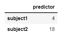
survival_functions = cph.predict_survival_function(X)
survival_functions

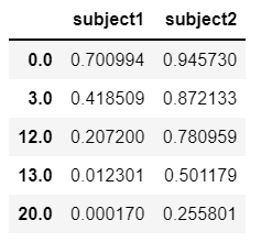
We now have a survival function for each subject. But these subjects are interested in the bottom line: how long before their symptoms return?

Calculating the expected value of lifespan as the area under the survival curve

The most common measure of central tendency for a continuous random variable is the expected value. The expected value of a random variable is the mean of its possible outcomes, weighted by their probability. Survival time is a continuous variable (although our petite example can be considered discrete), so we would need to integrate the function over the given range. This means that the expected value of the subject’s lifespan is the area under the survival curve.

Lifelines’ regression fitter objects have a method for calculating the expected value of the subject’s lifespan: predict_expectation(). It uses the trapezoidal rule to calculate the area under the curve.

cph.predict_expectation(X)

subject1 4.648343
subject2 13.456205
dtype: float64

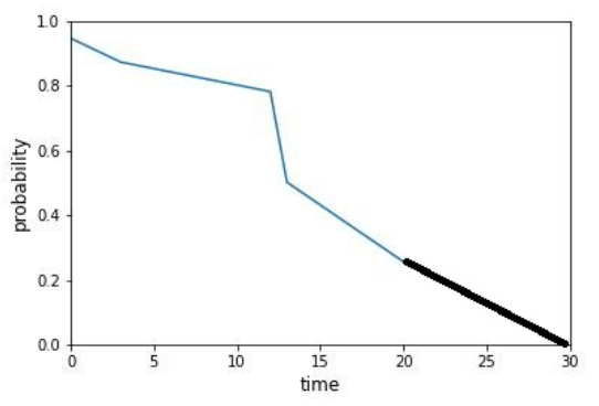
The documentation warns that “If the survival function doesn’t converge to 0, then the expectation is really infinity and the returned values are meaningless/too large”. Why is that? Let’s look at the survival function of subject no. 2, for example. Our predicted survival functions denote a probability for each of the durations the model trained on. For the latest time period, 20 days, subject 2 has a relatively high survival probability of 0.25.

import matplotlib.pyplot as plt

survival_functions['subject2'].plot()
xlabel = plt.xlabel("time")
ylabel = plt.ylabel("probability")
ylim = plt.ylim([0, 1])

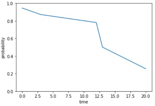
Calculating the area under the survival curve actually creates a downward bias as it is probable that the curve goes on after the 20th day. However, we don’t have enough information to determine how this function behaves for values larger than 20. There could be a substantial probability of a longer symptom-free period:

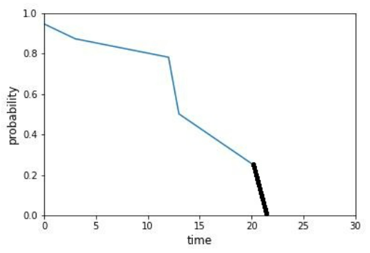
But it’s also possible that chances to ‘survive’ drop to zero straight after the 20th day.

Predicting the median lifetime

We’ve established that using the expected value for the time of symptoms recurrence, while mathematically beautiful, can be problematic. Instead, we can use the time at which the probability hits the 50% threshold as our prediction. Upon hitting this threshold, the probability that the event has not occurred becomes lower than the probability that it has occurred for every following time point. Using the median, or other percentiles, is simple and direct and is not affected by extreme values. Lifelines support this option directly through the predict_median() method.

cph.predict_median(X)

subject1 3.0
subject2 20.0
Name: 0.5, dtype: float64

It is no surprise that the median produces a different prediction than the expected value. Note that technically the function for subject no. 2 crosses the 0.5 thresholds on the 20th day, but it comes really close to crossing it on the 13th day. This is one of the pitfalls of a relatively crass survival function.

Nonetheless, it is not guaranteed that your survival function actually reaches the 50% probability! When your survival function predicts particularly high survival rates, the function may end before it even crosses the 50% mark, and the lifelines predict_median() method returns a value of inf. In such cases, it can be argued that predicting the time of symptom recurrence doesn’t make sense since the estimate, or the model, didn’t get enough relevant information. Let’s take a look:

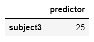
X2 = pd.DataFrame({"predictor": [25]}, index=['subject3'])
X2

cph.predict_survival_function(X2)

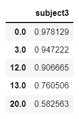
cph.predict_median(X2)

inf

Alternatively, if chances of survival are slim, the function may start from a probability lower than 0.5, and predict_median() will return a zero.

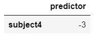
X3 = pd.DataFrame({"predictor": [-3]}, index=['subject4'])
X3

cph.predict_survival_function(X3)

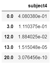
cph.predict_median(X3)

0.0

If you want to be on the safe side, depending on your use case, you can use a different percentile as the survival probability threshold value.

cph.predict_percentile(X, p=0.75)

subject1 0.0
subject2 13.0
Name: 0.75, dtype: float64

If you survived this post (see what I did there?), you are ready to take your survival function and turn it into a conclusive prediction. Keep in mind that the median is preferable to the expected value when the survival function doesn’t converge to zero, but it won’t save you if the function doesn’t even cross 0.5. Good luck!

---

Survival Analysis: Produce a Single Time-to-Event Prediction from Survival Functions was originally published in Towards AI on Medium, where people are continuing the conversation by highlighting and responding to this story.

Join thousands of data leaders on the AI newsletter. It’s free, we don’t spam, and we never share your email address. Keep up to date with the latest work in AI. From research to projects and ideas. If you are building an AI startup, an AI-related product, or a service, we invite you to consider becoming a sponsor.

Published via Towards AI