Step By Step Guide To Build Visual Inspection of Casting Products Using CNN

Author(s): Akshit Mehra

Originally published on Towards AI.

Introduction

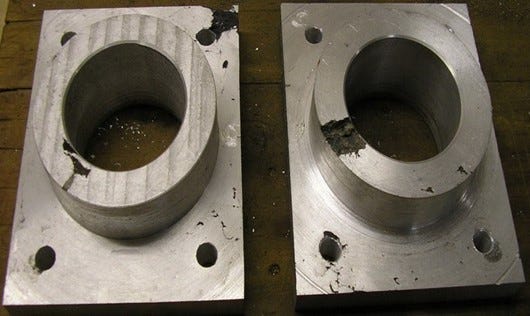
Casting refers to the manufacturing process in which a molten material like metal is poured into a hole or mold with the required shape and allowed to harden or solidify there. A casting defect refers to an irregularity introduced in the component during the casting process.

Figure: Casting Process (Source)

A quality inspection of these components becomes important because any defective product can cause the rejection of the whole order, which can cause a hefty financial loss to the business.

Instances where a defective product goes into the application is also undesired and is avoided at all costs. As it can cause some unexpected failure in the machine component, which can lead to huge losses.

Figure: Casting Defects (Source)

Visual Inspection of defects involves manually looking at each component and then deciding whether the piece is defective or not. This becomes both costly and time consuming.

In this blog, we try to use CNN (Convolution Neural Network), a deep learning model for detecting casting defects by analyzing images of casting products.

Prerequisites

To proceed further and understand CNN based approach for detecting casting defects, one should be familiar with:

1. Python: All the below code will be written using python.
2. Tensorflow: TensorFlow is a free and open-source machine learning and artificial intelligence software library. It can be utilized for a variety of tasks, but it is most commonly employed for deep neural network training and inference.
3. Keras: Keras is a Python interface for artificial neural networks and is an open-source software. Keras serves as an interface for the TensorFlow library
4. Jupyter Notebook: Jupyter notebooks are web-based platforms built for mathematical and scientific computations. We build our tutorial on jupyter Notebook.

Apart from above listed tools, there are certain other theoretical concepts one should be familiar with to understand the below tutorial.

1. Convolution Neural Networks

Convolution Neural Networks (CNN) are a type of network architecture in deep learning which are mainly used for image related tasks, like Image classification, Image segmentation, etc. The network connectivity in CNN resembles that of the human brain.

Figure: Convolution Neural Network Architecture

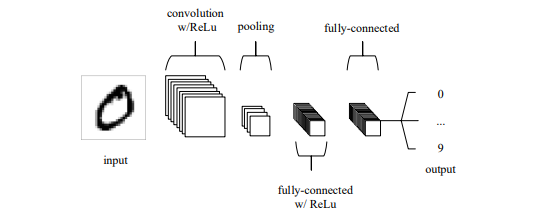
Convolution Neural Network are composed mainly of 3 layers:

1. Convolution Layer: The convolutional layer will calculate the scalar product between the weights of the input volume-connected area and the neurons whose output is related to particular regions of the input.
2. Pooling Layer: To further reduce the amount of parameters in that activation, the pooling layer will then simply down-sample along the spatial dimensionality of the input.
3. Fully Connected Layers: The fully-connected layers will next carry out the similar tasks as in conventional ANNs and make an effort to derive class scores from the activations, which can subsequently be used for classification.

One of the major advantages of using CNN is Parameter sharing. The idea behind parameter sharing is that if a region characteristic can be computed at one specific spatial location, it is likely to be helpful at another.

The output volume’s total number of parameters will be drastically reduced if each individual activation map is constrained to have the same weights and bias.

2. Activation functions

Generally, the data that we work on is non linear in nature, i.e. the instance features and the corresponding prediction value. Activation functions are functions which are applied to each neuron/cell in artificial neural networks to introduce non-linearity in them.

There are many activation functions which are used:

1. ReLU: ReLU basically stands for Rectified Linear unit. Mathematically, it is defined as:

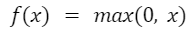Figure: Mathematical Formuale for ReLU

The ReLU activation function is far more computationally efficient as compared to other

activation functions. Further, it converges faster to the global minimum due to its linearity and non saturating nature.

1. Sigmoid: Sigmoid function, also known as logistic function, takes input any real value and outputs a value in the range of 0 to 1. It is one of the most widely used activation functions. Mathematically, it is represented as

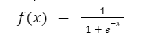Figure: Mathematical Formulae for sigmoid function

This function is generally used for models where output computed is the probability.

Also, the function is differentiable and thus forms a smooth gradient, i.e it prevents the output values from jumping around or causing oscillations.

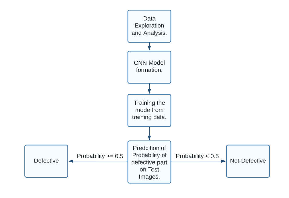
Methodology

To proceed further with our CNN based inspection system:

1. We start with a data exploration task. We analyze the data and figure out if any skewness, or if any pattern is observed.
2. Create our CNN model using Tensorflow and train it using training data.
3. Perform hyperparameter tuning to fine tune our model, i.e. reduce overfitting or underfitting.
4. Perform prediction on test Images.

Figure: Flowchart for methodology (Image by author)

Dataset Selection

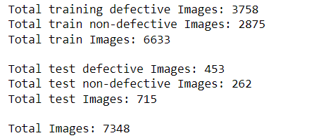
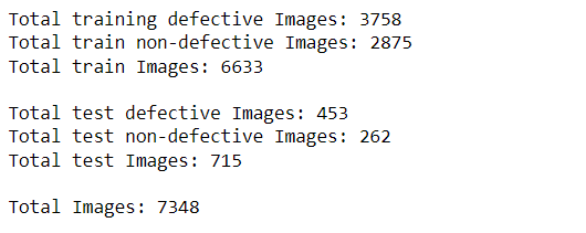
For our project, we will use the dataset available on Kaggle. The dataset contains images of defective and non-defective parts. In total there are 7358 images out of which 6633 training images and 715 test images. Further breaking down,

Figure: Analysis of dataset (Image by author)

The images are 3 channel images, i.e. RGB in nature with a dimension of (300, 300, 3).

Implementation

Now, we will begin to code for a CNN based system for detecting casting defects.

Environment Setup

Below points need to be done before running the code:

1. The code below is written in my local jupyter notebook. Therefore, install jupyter. You can refer to this https://www.anaconda.com/products/distribution. You can install anaconda and use jupyter from there.
2. If Anaconda doesn’t work, you can refer to: https://jupyter.org/install.
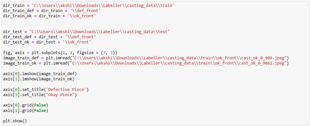
3. The Datadirectory variable contains a path to the folder containing image data.

It is a path to the directory which contains the path to both folders, train and test.

4. Further, test and train directory are divided into 2 folders i.e. ok_front which contains non-defective images of components and def_front which contains images of defected parts

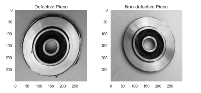
Hands-on with Code

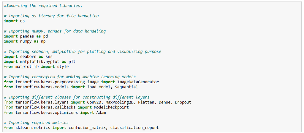
We begin by importing all the required libraries.

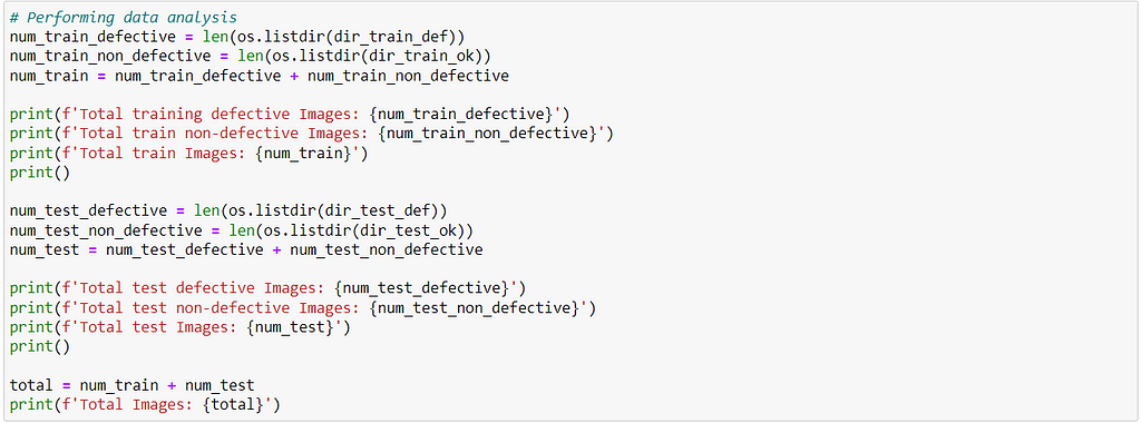
Next, we perform a data visualization. The dataset contains a total of 7448 images of both defective and non-defective. We basically plot a histogram comparing number of images which are defective vs non-defective.

We also do a bar plot to see a comparison between defective and non-defective data to see if data contains any skewness.

Figure: Barplot comparing count of Defective and Non-defective (Image by author)

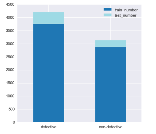
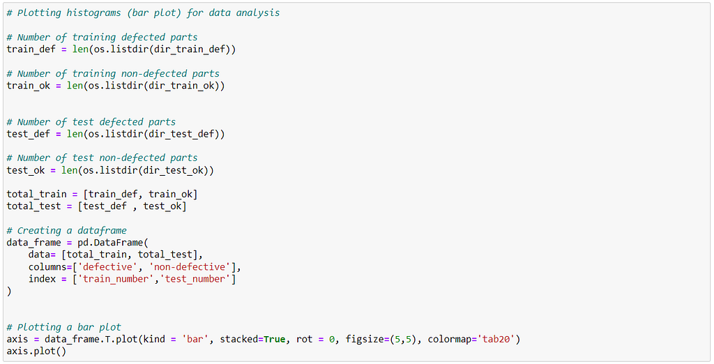
From the above plot, we see that the dataset is a bit skewed towards defective parts. But, the data is distributed such that 60% of images are defective and 40% are non-defective. Thus, in this case the model will not be that biased.

But in cases where the data is largely skewed towards some class, it could result in the model being biased towards that particular class. In such case, one can:

1. Increase the dataset so that skewness reduces.
2. Perform data augmentation on the existing dataset.

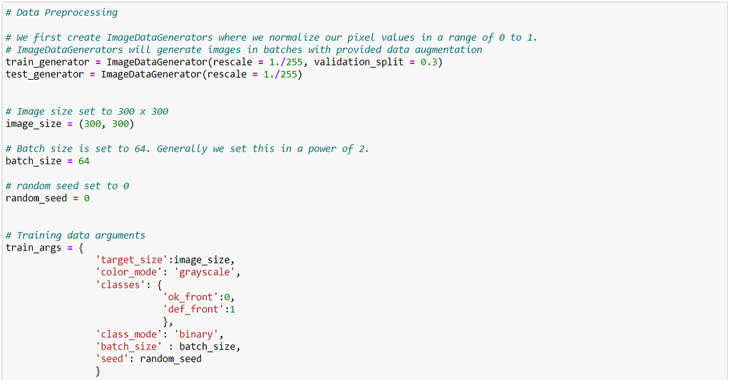
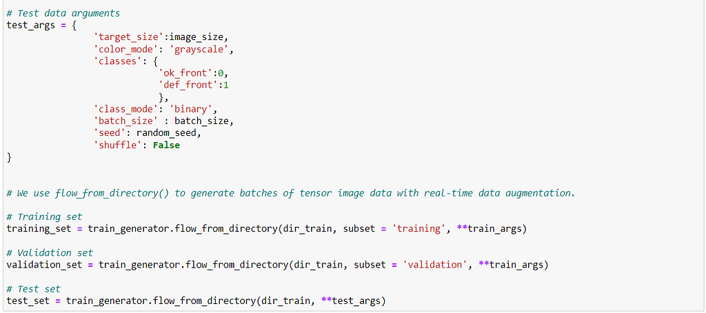
Next, we do some data preprocessing.

Here,

1. We normalize the pixel values in the range of 0 to 1. For this, we divide our pixel values by 255.
2. Resize our images to (300 x 300) , i.e. to grayscale mode.
3. Set the batch size to 64. Batch size is set because images are trained in batches. This improves the model while training.
4. Set the class mode to binary, as we only have 2 classes.
5. Set 30% of our training data as validation data.

Why did we normalize the pixel values before using them for training?

The normalization of pixel values was done to prevent overflow of weight during the backpropagation. During backpropagation, chain rule is followed according to which the pixel values keep on getting multiplied as we update initial layer neurons.

Thus, the weight values can easily overflow, i.e. become very large which makes them computationally inefficient.

Why is the batch size chosen to be 64?

Generally, batch sizes are chosen in the power of 2 to fully utilize the capacity of GPU’s processing. In most cases, it is either 32 or 64.

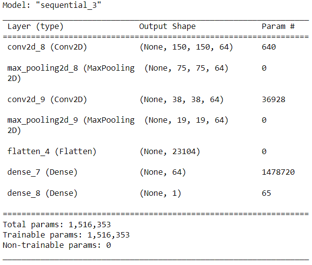
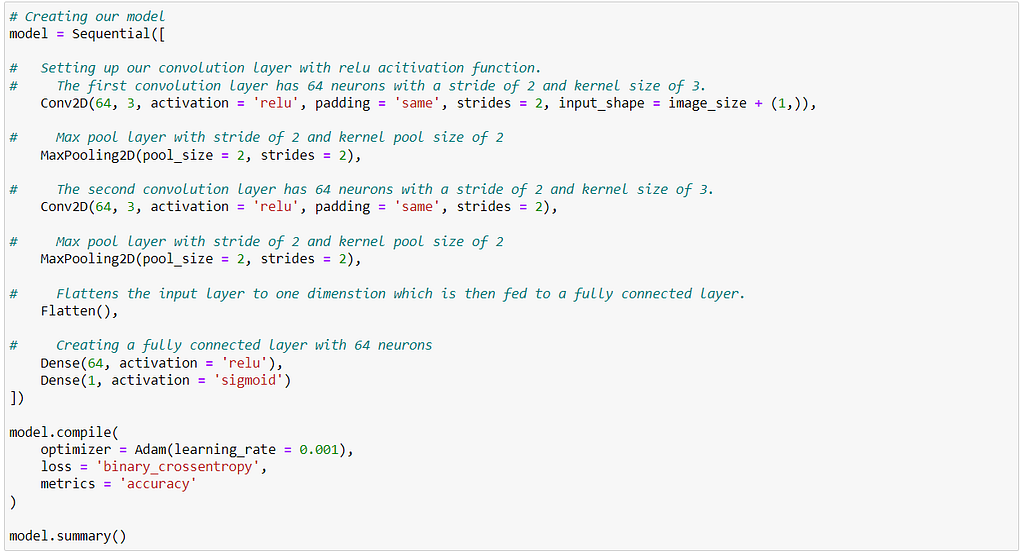
Next, we create our model. The model used contains:

1. 2 Convolution layers, each of which is followed by a Max pooling layer.
2. Each convolution layer has a ‘Relu’ activation layer.
3. A fully connected layer having 128 input cells.
4. A final layer with one neuron which predicts the probability of a component being defective. Here, the sigmoid activation function is used.

Figure: Model Summary (Image by author)

In the next step, we start training our model.

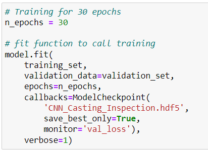
While training our model:

1. We monitor the validation loss.
2. The model is saved after training as ‘CNN_Casting_Inspection.hdf5’ so it can be used later.

Why did we train the model for 15 epochs?

After training the model for 15 epochs, there wasn’t any significant change in both accuracy and the validation loss. Thus, if we would train for more epochs, it would eventually lead to overfitting in model.

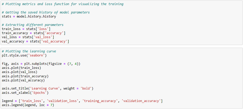
After we have trained our model, we visualize the training of it using different plots, which includes plotting:

1. Training loss
2. Validation loss
3. Training accuracy
4. Validation accuracy

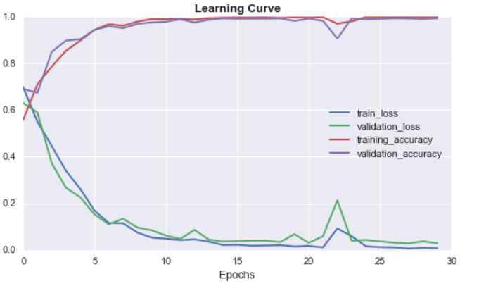
From the above plot, we see that with increasing epochs:

1. Both validation and training loss decreases.
2. Both validation and training accuracy increases.

The loss plot does not have much oscillation which indicates that the learning rate used is good enough.

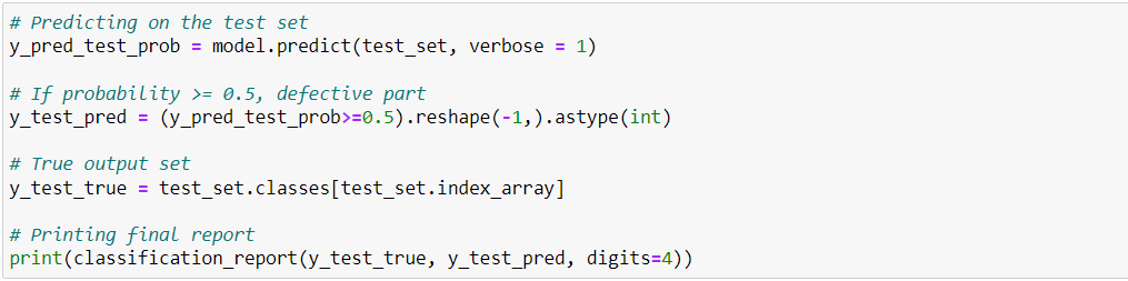
Finally, we predict the output on test images. We print the results for test images using classification_report() function from scikit_learn.

Figure: Final classification report

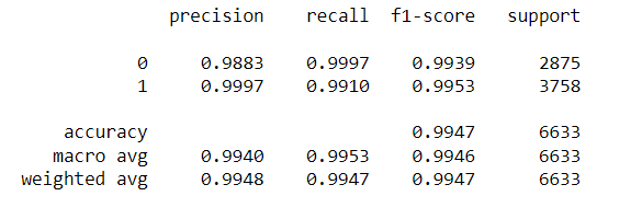
The final model accuracy is 99.47, which is pretty good.

If we see the task of inspecting individual images of components to detect casting defects, we would want to:

1. Eliminate the false negatives, i.e. instances when a defected part goes into production.
2. Eliminate the false positives, i.e. instances when a non-defective part is detected to be defected.

Thus, we would want to monitor f1-score closely as compared to accuracy, precision or recall.

The observed f1-score:

1. 0.9939 for class 0, i.e. non-defected.
2. 0.9953 for class 1, i.e. defected.

Conclusion

In this blog, we performed the task of visually inspecting casting products by analyzing their images using a class of deep learning architectures known as Convolution Neural Networks. The important points include:

1. We begin by first analyzing the data, i.e. plotting the images, their count, dimensions, etc.
2. We then performed some data-preprocessing, like:
3. Changing image dimensions
4. Changing image to gray-scale
5. Rescaling pixel values between 0–1.
6. Next, we create our model. The model has 2 convolutional layers each followed by a MaxPooling layer. At the end, we then have a fully connected layer followed by a final layer where output is predicted.
7. We finally predicted our output on test images.

The task performed above was basically Image classification only, where we had 2 classes Defective and Non-defective. Similar to this, any Image classification task can be performed using the above approach.

References

1. https://arxiv.org/pdf/1511.08458.pdf
2. https://medium.com/r?url=https%3A%2F%2Fengmag.in%2Findian-casting-industry-poised-for-significant-growth-in-performance%2F
3. https://medium.com/r?url=https%3A%2F%2Fwww.rapiddirect.com%2Fblog%2F17-types-of-casting-defects%2F

---

Step By Step Guide To Build Visual Inspection of Casting Products Using CNN was originally published in Towards AI on Medium, where people are continuing the conversation by highlighting and responding to this story.

Join thousands of data leaders on the AI newsletter. Join over 80,000 subscribers and keep up to date with the latest developments in AI. From research to projects and ideas. If you are building an AI startup, an AI-related product, or a service, we invite you to consider becoming a sponsor.

Published via Towards AI