Sound and Acoustic patterns to diagnose COVID [Part 3]

Author(s): Himanshu Pareek

Originally published on Towards AI the World’s Leading AI and Technology News and Media Company. If you are building an AI-related product or service, we invite you to consider becoming an AI sponsor. At Towards AI, we help scale AI and technology startups. Let us help you unleash your technology to the masses.

Link to part 1 of this case study

Link to part 2 of this case study

In the last part we built some models on our train data and calculated metrics on our test data.

Bayesian optimization and Hyperopt:

Hyperopt is a tool that finds the best model and hyperparameters based on Bayesian optimization and SMBO (sequential Model-based global optimization). Essentially, with Bayesian optimization, it finds P(score|configuration) — the probability of score given a certain configuration, for different configurations and then determines the best one. This configuration can be a model with different values for hyperparameters or different models with different hyperparameters. Using Bayesian optimization, the algorithm is able to narrow down the search space to find these configurations and provide the result faster.

I have used this tool to find the best model and parameters for our data set and then implemented it.

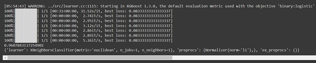
According to the above, the best model is KNN, with Euclidean distance and K=1. It is also suggested to use L1 normalization as a preprocessing step.

K-Nearest Neighbors:

In KNN, neighbors of the query point are found in the dataset, and the class label of the majority of the neighbors is given as the class label for the query point. below is the result.

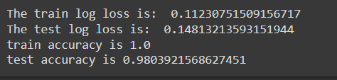
The model produced a train log loss of 0.11 and a test log loss of 0.14. The training accuracy is 100 percent, while test accuracy is 98 percent. It is noteworthy that the difference in loss between train and test loss is less, suggesting the model has not to overfit.

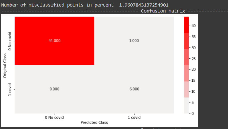
From the below confusion matrix plot, it can be observed that all positive points are correctly classified, while one negative point is incorrectly classified in the test data.

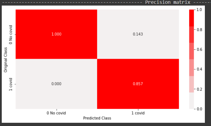
From the above precision plot, it can be concluded that 85 percent of the predicted positives were actual positives, and 100 percent of the predicted negatives were actual negatives.

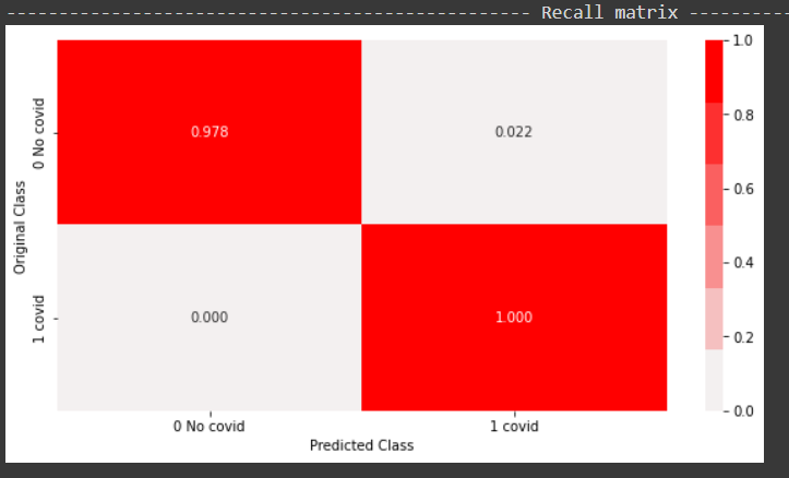
From the above recall plot, it can be concluded that the positive class has 100 percent recall, while the negative class has 97 percent recall.

This concludes the classical machine learning implementations for our problem. In conclusion, KNN performed the best. There is more scope for hyperparameter tuning and getting better results, however, it is clear that classical techniques can classify our data in a very limited capacity and there is a good chance of overfitting to training data.

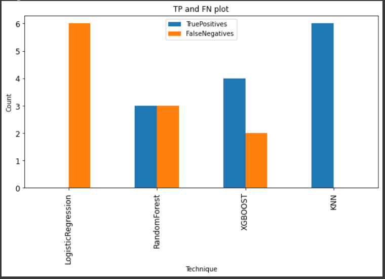
Now, since the problem is that of medical diagnosis, the important metrics for us are the True positive rate and the false-negative rate. It is important to reduce the FNs and increase the TPs.

Below is the plot for TP and FN for all the above models.

Deep learning-based models

Next, we will implement some deep learning models and analyze their performance.

Convolution neural network

A kernel is used to convolve over the image pixel by pixel and the dot product is stored in another matrix, which is the result of this convolution. Many such layers of convolution are used to learn from the input image. In our case, the image is a sound spectrogram that was discussed in detail earlier. All our dataset is converted into spectrograms. CNN is used over these spectrograms, followed by a binary classification layer, to make predictions on whether the spectrogram belongs to a covid positive or covid negative sound.

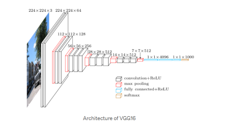
VGGNet:

This is convolution-based architecture. Only 3×3 kernels are used for the entire architecture, and 2×2 max pooling is used with stride 2. This immensely simplifies this architecture. VGG 16 has 16 layers. This is being used for transfer learning for our task. In Keras, there is a pre-built VGG 16 model trained on imagenet dataset.

Transfer learning refers to re-using a pre-trained model for the current job instead of building the model from scratch. If we remove the top layers, which are flattened and fully connected dense layers, the output received is the bottleneck features. The weights of the initial layers are frozen, so gradients do not pass through them, and the weights are not updated. Fine-tuning means using a lower learning rate, so weights are not updated drastically.

In our task, both bottleneck and fine-tuning will be applied to see the results.

CNN Model 1:

The image data generator and the flow from the data frame method are used to prepare our images for training. After doing the test train split, we get 30 percent images in the validation set and 70 percent in the train set. For the first task of using bottleneck features, the target size of the images used is that of the original spectrograms, which is 288×432. With shuffle as true, the class mode used is binary as our task is of binary classification.

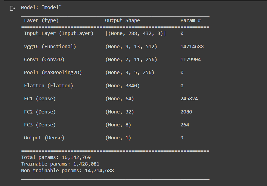
In the final model, there is an input layer, then the VGG 16 model with the top removed. The weights are frozen here. Weights are initialized with the imagenet data set. We have a convolution layer, a pooling layer followed by flattened and dense layers. In the end, we have a single sigmoid neuron for binary classification.

Model is compiled with Adam optimizer with a learning rate of 0.01, binary cross-entropy loss, and a set of metrics. The metrics include binary accuracy, TP, FP, TN, FN.

The model was trained for 50 epochs.

30/30 [==============================] — 13s 433ms/step — loss: 3.9778e-07 — binary_accuracy: 1.0000 — tp: 11.0000 — tn: 108.0000 — fp: 0.0000e+00 — fn: 0.0000e+00 — val_loss: 0.8592 — val_binary_accuracy: 0.9412 — val_tp: 5.0000 — val_tn: 43.0000 — val_fp: 0.0000e+00 — val_fn: 3.0000

<keras.callbacks.History at 0x7f955de702d0>

The model produced an accuracy of 100 percent for the training set. A 0.94 accuracy for the validation set with 3 false negatives in total.

CNN Model 2:

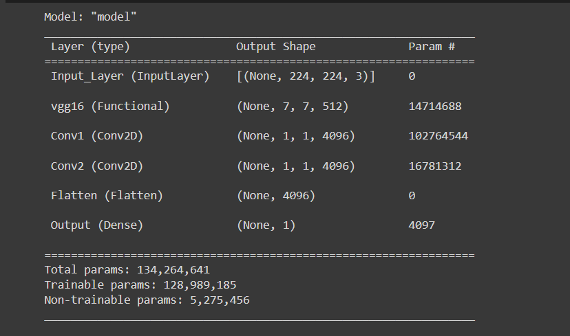
For the second task of fine-tuning the VGG 16 model for transfer learning, the images are resized to 224×224, which is the standard input size of the VGG-16 model. With shuffle as true, the class mode used is binary as our task is of binary classification.

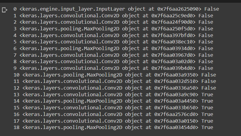
In this model, the base model is VGG 16. We have frozen the initial layers of this model but did not freeze the later layers. 6 layers are not frozen.

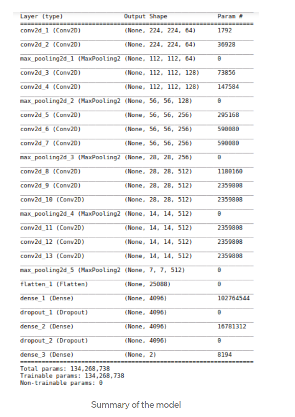
The final model contains the input layer, VGG 16 described above followed by 2 convolution layers. Here convolution layers are used instead for fully connected layers. This speeds up the training. Then there is a flatten layer, followed by the output layer of sigmoid activation. There are approximately 130 million trainable parameters in this network.

While compiling this model, we have used the concept of reducing the learning rate. We used the Adam optimizer with a lower learning rate of 0.0001. We also used the same metrics described previously. Using reducing learning rate with a minimum of 0.000001.

Epoch 50/50

30/30 [==============================] — 16s 531ms/step — loss: 4.6876e-07 — binary_accuracy: 1.0000 — tp: 16.0000 — tn: 103.0000 — fp: 0.0000e+00 — fn: 0.0000e+00 — val_loss: 0.1338 — val_binary_accuracy: 0.9608 — val_tp: 2.0000 — val_tn: 47.0000 — val_fp: 1.0000 — val_fn: 1.0000 — lr: 1.0000e-06

<keras.callbacks.History at 0x7f6aa02ca7d0>

As seen above, we trained the model for 50 epochs. An accuracy of 100 percent on the train set and an accuracy of 96 percent on the validation set are obtained. However, the false-negative is only 1, and the false-positive is 1. This is much better than the CNN model 1 as we care most about reducing FN and increasing TP, which was achieved in this model.

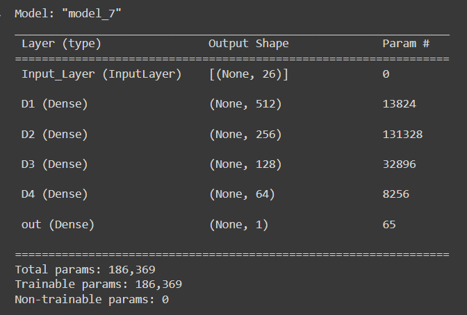
Multilayered Perceptron

A multilayered perceptron was built with 4 dense layers, an input layer, and an output layer. The output consists of 1 sigmoid unit as our task is that of binary classification. As metrics, binary accuracy and confusion matrix components are used. Binary cross-entropy is used as a loss function. Adam optimizer is used as an optimizer with 0.01 as the learning rate.

Here we have used the tabular features that were used for classical machine learning models.

Below is the model summary. Our model has around 186,000 trainable parameters.

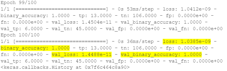
As observed above, the model was trained for 100 epochs and the loss at the end is very low. A 100 percent train and validation accuracy was achieved with this model.

However, for a holistic view of the results, we need to train and test the above model on multiple train/test splits of the data.

Rerunning the MLP based model, using several train test splits, to understand average performance

In this experiment, multiple train test splits were created and an MLP model was run on them. The performance metrics were captured and recorded.

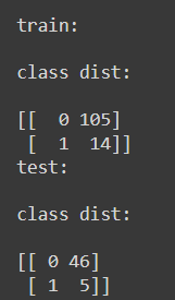
As observed above, this is the first run of 5 runs, wherein in the train data set we have 14 positive points while in the test dataset, we have 5 positive points. After running the model for 100 epochs, the test loss was 0.014, accuracy was 100 percent.

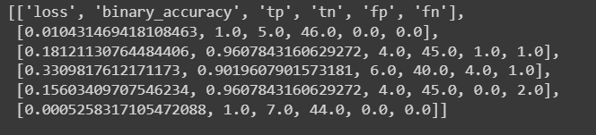
A similar process was repeated 5 times on different train test splits. Below is the final result. As observed, the accuracy is above 90, and close to 100 in many runs. More importantly, we have low false negatives and high true positives.

Thus, we will move ahead with this model as the final model and productionize it.

Deployment and Productionisation

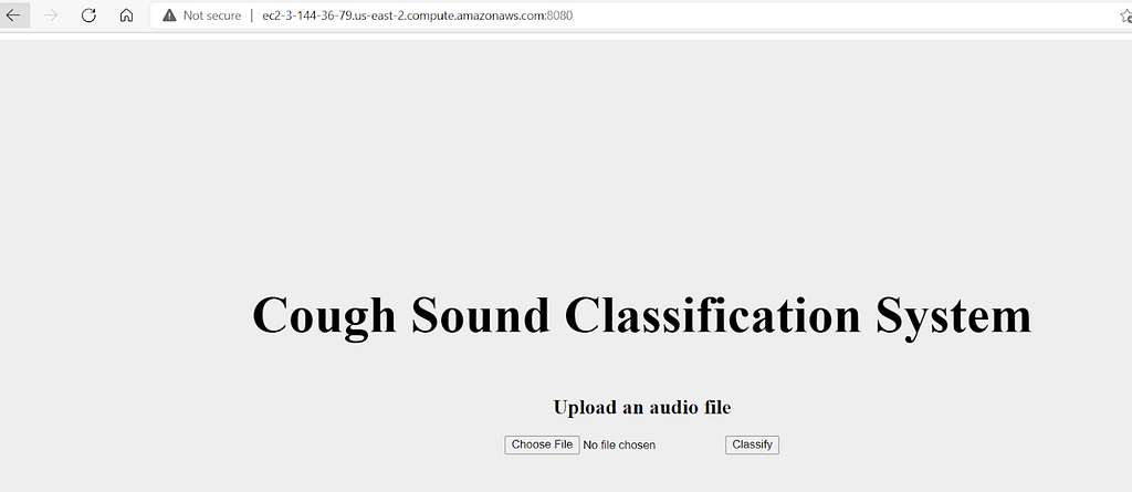
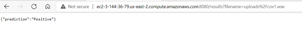
The final model used is a deep learning MLP model. The two key files needed for deployment and product ionization are the saved model file and the pickle file for data standardization. An API is created around the model that takes in the audio file as an input and returns the label as output. The output is in JSON format.

The UI is simple. The file is uploaded and the classify button is clicked. This will post the file to the server and a class label will be returned back to the client. This is achieved using the flask API module.

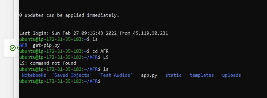
We will use the AWS cloud for deploying this application. We will use an elastic cloud compute service. First, an EC2 instance will be launched and required libraries are installed. Then using a secure copy, we will transfer the required files from the local to the EC2 box. Then run the app.py file on the EC2 server.

Conclusion

In this case study, we attempted to create a working model that could classify cough sounds. Even with a small dataset, the results were good and promising. Both classical machine learning methods and deep learning methods were employed. In classical methods, KNN gave the best results. To find the best model, we also utilized Bayesian optimization.

In deep learning methods, multi-layer perceptron and convolution neural networks were implemented. For classical methods and MLP, we used tabular data. The data was engineered from the time series of the audio signal. For CNN, we used spectrograms.

As a final model, we chose MLP as it gave good results and is faster to train. It has a comparatively low prediction time and low prediction cost when compared to CNN.

The model was deployed on the AWS EC2 service. Around the model, an API was developed using Flask.

Hope you enjoyed reading it!!

---

Sound and Acoustic patterns to diagnose COVID [Part 3] was originally published in Towards AI on Medium, where people are continuing the conversation by highlighting and responding to this story.

Join thousands of data leaders on the AI newsletter. It’s free, we don’t spam, and we never share your email address. Keep up to date with the latest work in AI. From research to projects and ideas. If you are building an AI startup, an AI-related product, or a service, we invite you to consider becoming a sponsor.

Published via Towards AI