Reinforcement Learning: Monte-Carlo Learning

Author(s): blackburn

Originally published on Towards AI the World’s Leading AI and Technology News and Media Company. If you are building an AI-related product or service, we invite you to consider becoming an AI sponsor. At Towards AI, we help scale AI and technology startups. Let us help you unleash your technology to the masses.

Model-free learning.

In the preceding three blogs, we talked about how we formulate an RL problem as MDPs and solve them using Dynamic Programming (Value iteration and Policy iteration). Everything we have seen so far deals with the environments we had full knowledge about i.e.transition probability, reward function etc. A natural question would be, what about the environments in which we don’t have the luxury of these functions and probabilities? This is where a different class of reinforcement learning known as Model-free learning comes in. In this blog, we will learn about one such type of model-free algorithm called Monte-Carlo Methods. So, before we start, let’s look at what we are going to talk about in this story:

• Basic Intuition of Monte-Carlo
• Calculating Mean on the go i.e. Incremental Means
• How do we evaluate a policy in Model-free environments? (policy evaluation)
• The problem of exploration…
• On-policy policy improvement(control)
• What is GLIE Monte-Carlo?
• Important Sampling
• Off-policy policy improvement(control)

This is gonna be a long ride, so make yourself a coffee and sit tight!☕🐱‍🏍

Basic Intuition of Monte-Carlo

Monte Carlo(MC) method involves learning from experience. What does that mean? It means learning through sequences of states, actions, and rewards. Suppose, our agent is in state s1, takes an action a1, gets a reward of r1, and is moved to state s2. This whole sequence is an experience.

Now, we know that the Bellman equation describes a value of a state as the immediate reward plus the value of the next state. As for our case, we don’t know the model dynamics(transition probabilities) so we cannot calculate this. But if we look at environments where we don’t have knowledge about environment dynamics and ask ourselves what we still know(or can know) about the environment is the rewards. If we take the average of these rewards and repeat this infinite times then we can estimate the value of the state close to the actual value. Striking! Monte Carlo is all about learning from averaging the reward obtained in these sequences. So, to put it…

Monte Carlo involves learning through sampling rewards from the environment and averaging over those obtained rewards. For every episode, our agent takes action and obtains rewards. When each episode(experience) terminates then we take the average.

This raises a question, do we average over the reward every time we visit the state in an episode? Well yes and no. Explanation: In an episode, if we only average over the rewards obtained after state s was visited for the first time then it is called First-visit Monte Carlo, and if in an episode, we average over the rewards obtained every time state s is visited we call it Every-visit Monte Carlo. Mostly in this blog, we will be talking about First-visit MC.

This describes the crux of MC. But it leaves a lot of questions unanswered like how do we make sure that all states are visited? or how to calculate the mean efficiently? In the remaining blog, we are just gonna build upon this idea. Let’s learn about one such idea i.e. Incremental Means.

Incremental Means

As described before, to calculate the value function of the state (s) we average over the rewards obtained after visiting that state (s). This is how it is described:

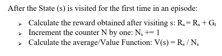
You might ask if we are calculating reward only the first time state s was visited in an episode then the counter N will always be 1. No, as this counter assists us over every episode the state s was visited.

Moving forward we might want to calculate the rewards and average them incrementally rather than summing all the rewards at once and dividing them. Why? Because keeping the sum of all the rewards and then dividing it by the total number of times that state was visited is computationally expensive and this requirement will grow as more rewards are encountered. We will have to assign more memory every time a new state/reward is encountered. Therefore, here we define derivation for incremental means.

Incremental means: Also known as moving averages, it maintains the mean incrementally i.e. the mean is calculated as soon as new reward is encountered. In order to calculate inremental mean, we don’t wait till every reward is encountered and then divide it by the total number of times that state was visited. We calculate it in an online fashion.

Let’s derive incremental means step-by-step:

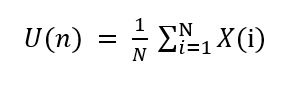
▹ The total mean for n time steps is calculated as :

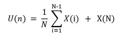
▹ Let’s say, U(n) is the new mean we want to calculate. Then this U(N) can be split into the sum of the previous mean till N-1 and the value obtained at N timestep. Can be written as:

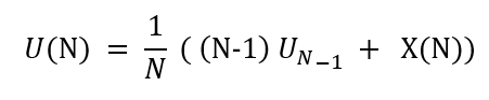
▹ Now looking at the summation term, it can be defined as (N-1) times the mean obtained till N-1 i.e. U(N-1). Substituting this in the above equation:

▹Rearranging these terms :

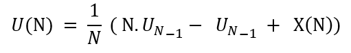
▹Taking N common and Solving further:

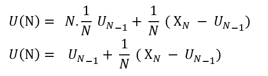
What does this equation tell us?

It tells that the new mean (U(N)) can be defined as the sum of the previous estimate of the mean (U(N-1)) and the difference between the current obtained return (X(N)) and the previous estimate of the mean (U(N-1)) weighted by some step size i.e. the total number of times a state was encountered over different episodes. The difference between the current obtained return (X(N)) and the previous estimate of the mean (U(N-1)) is called the error term and it means that we are just estimating our new mean in direction of this error term. It is important to note that we are not accurately calculating the new mean but just pushing the new mean in the direction of the real mean.

So, that sums up incremental means.😤 Now, let’s dive deeper into how we evaluate/predict a policy in MC.

Policy Evaluation in Model Free Environments (for MC)

Policy Evaluation is done as we discussed above. Let’s elaborate on it. Recall that, the value function is calculated by averaging the rewards obtained over episodes. So, the next question will be how do we construct/extract a policy from this value function. Let’s have a quick look at how policy is constructed from state-value function and state-action value(Q-Function).

Mathematically, the policy can be extracted from the state-value function:

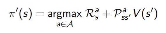
As we can see that to extract a policy from the state-value function we maximize the state values. But this equation has two problems. First, in the model-free environment, we don’t know transition probabilities(Pss’), and second, we also don’t know s’.

Now, let’s look at the state-action function. The policy is extracted as :

As we can see, we only need to maximize over the Q-values to extract the policy i.e. we maximize over the actions and choose the action which gives the best Q-value(state-action value). So, for MC we use the state-action value for policy evaluation and improvement steps.

How do we calculate state-action values? Well, we calculate the action-values same as we do for state-values only difference is that now we calculate it for every state-action pair (s, a) rather than just state s. So, a state-action pair (s, a) is said to be visited only if state s is visited and action a is taken from it. We average over the action values as described in the previous section and that gives us the state-action value for that state. If we average only after the (s, a) pair was visited for the first time in every episode then it is called First-visit MC and if we average over (s, a) after every visit to it in an episode then is called Every-visit MC.

So, averaging over state-action values gives us the mechanism for policy evaluation and improvement. But it also has one drawback i.e. the problem of exploration. Let’s take care of that too.

The problem of exploration

For the policy evaluation step, we run a bunch of episodes and for each episode, we calculate the state-action values for every (s, a) pair we encountered then we take an average of these, and that defines the value for that (s, a) pair. Then we act greedy as our policy improvement step w.r.t. to state-action values. Everything looks good but wait! If we act greedy as our policy improvement step then there will be many state-action pairs we might never visit. If we don’t visit them then we will have nothing to average and their state values will be 0. This means that we might never know how good that state-action pair was. This is the problem we will try to solve in this session. What kind of policy is adequate for MC?

Well, we desire a policy that is generally stochastic π(a|s) > 0, meaning that it has a non-zero probability of selecting any action for all states, and then gradually changes to a deterministic policy as it approaches optimality. Initially, being stochastic and having π(a|s) > 0 for all actions will ensure that all actions have an equal chance of being selected in a state which will ensure exploration and then gradually shifted to deterministic policy because an optimal policy will always be a deterministic one that takes the best action possible of all actions in a state. This policy ensures that we continue to visit different state-action pairs.

This can be done using two approaches i.e. On-policy methods and Off-policy methods. Both of which are discussed in the following sections.

Monte Carlo Control

MC control is similar to what we saw for solving Markov-decision processes using dynamic programming(here). We follow the same idea of generalized policy iteration (GPI), where we don’t directly try to estimate optimal policy instead we just keep an estimate of action-value function and policy. Then, we continuously nudge the action-value function to be a better approximation for the policy and vice-versa (see previous blogs). This idea can be expressed as:

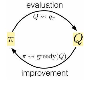
In MC, we start with some policy π and use it to calculate the action values. Once the action-values are computed(policy evaluation) then act greedy with respect to these action-values(control) to construct a new policy π*, which is better or equal to the initial policy π. Oscillating between these two steps ultimately yields an optimal policy.

On-policy control

In the On-policy method, we improve the same policy which is used for evaluating the Q-function. Intuitively, suppose we evaluate a state-action value(Q-function) for a state s using a policy π then in the policy control we will improve this same policy π. The policies used in the on-policy method are the epsilon-greedy policies. So, what is an epsilon-greedy policy?

As described in the previous section, the desired policy for MC is π(a|s) > 0 and this type of policy is called the epsilon-soft policy. The policy used in on-policy is called ϵ-greedy policy. This type of policy has a probability of selecting a greedy action with a probability of 1- ϵ + ϵ/A(s) and taking a random action with a probability of ϵ/A(s), where A(s) is the total number of actions that can be taken from that state. It can be expressed as:

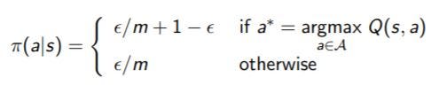
For ϵ-greedy policy, each action has a π(a|s) >ϵ/A(s) probability of being selected. An ϵ-greedy policy selects greedy action most of the time but with a slight probability, it also selects a completely random action. This solves our problem of exploration.

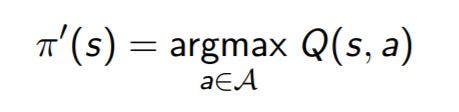
Now, we can improve the policy by acting greedy i.e. by taking the action that has a maximum q-value for a state. This is given as(we saw this earlier):

Building along the ideas of GPI the evaluation and improvement step is done till optimality is achieved as shown below.

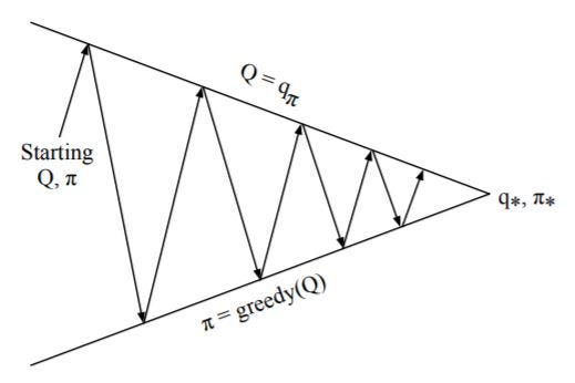
But recall that, GPI doesn’t necessarily require that policy evaluation be done for one complete pass instead we can evaluate a policy for one episode and then act greedy to it. It only requires that the action values and policy are nudged a little towards optimal action values and optimal policy as denoted below:

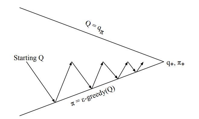
Combining all the mechanisms we just saw, we can present an on-policy algorithm called Greedy in the Limit with Infinite Exploration(GLIE).

Greedy in the Limit with Infinite Exploration

Everything up till now has been leading to this algorithm. As discussed earlier, the ideal formulation of policy for MC will be:

1. We keep on exploring, meaning that every state-action pair is visited an infinite number of times.
2. Eventually, later steps shift towards a more greedy policy i.e. deterministic policy.

This is assured by setting the right values for ϵ in the ϵ-greedy policy. So what are the right values for ϵ?

Initial policy is usually some randomly initialized values so to make sure we explore more and this can be ensured if we keep the value of ϵ~1. In the later time-steps we desire a more deterministic policy, this can be ensured by setting ϵ~0.

How does GLIE MC set the ϵ value?

In GLIE MC, the ϵ value is gradually decayed meaning that the value of the epsilon becomes smaller and smaller with each time-steps. Usually, the practice is to with an epsilon value = 1.0 and then slowly decay the epsilon value by some small amount. The value of ϵ >0 will mean a greedy policy is followed. So, in GLIE Monte-Carlo ϵ value is gradually reduced to favor exploitation over exploration over many time steps.

Next, we look into important sampling which is at the crux of off-policy MC.

Important Sampling

In Off-policy, we have two policies i.e. a behavior policy and a target policy. The behavior policy is used to explore the environment. It generally follows an exploratory policy. The target policy is the one we want to improve to optimal policy by learning the value function based on behavior policy. So, the goal is to learn the target policy distribution π(a/s) by calculating the value function derived from the samples from behavior policy distribution b(a/s). Important sampling helps in just that. Detailed explanation :

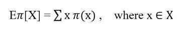
Let’s say we want to estimate the expected value of random variable x where x is sampled from behavior policy distribution b [x ~b] w.r.t to the target policy distribution π i.e. Eπ[X]. We know that:

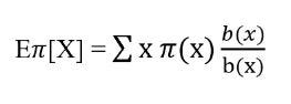
Dividing and multiplying by behavior distribution b(x):

Re-arranging the terms:

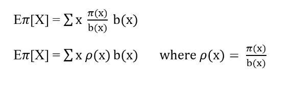
In equation 3, the ratio between x~target policy distribution and x~behavior policy distribution is called an important sampling ratio denoted by p. Now the expectation for π is from b. There are two ways we can use important sampling to calculate the state-value function for target policy i.e. Ordinary Important sampling and Weighted important sampling.

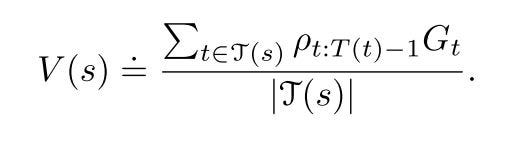
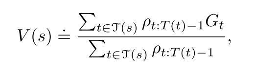
Ordinary important sampling keeps track of time steps in which a state was visited denoted by T(s). The Vπ is the result of scaling the returns obtained from behavior policy and then dividing it by T(s).

On the other hand, Weighted important sampling is defined as the weighted average as follows:

Ordinary important sampling is unbiased whereas weighted important sampling is biased. What do we mean by that? Well, suppose if we only sample a single return from a state then in weighted important sampling the ratio terms in numerator and denominator will cancel out. Therefore the estimate Vπ will be the returns from behavior policy b without any scaling. This means that its expectation is not Vπ but is Vb. On the flip side, the variance of ordinary important sampling is unbounded whereas this is not the case for weighted important sampling. This sums up important sampling.

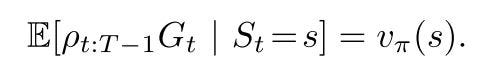
Off-Policy Monte Carlo

As mentioned previously, we want to estimate the target policy from the behavior policy. As in MC, we estimate the value of the state by averaging the returns. We are going to do the same here. We calculate the value function by estimating the returns as follows:

where p is the important sampling ratio defined as the probability of a certain trajectory under π divided by the probability of a certain trajectory under b. Recall that the trajectory under policy π is defined as the probability of taking an action a in state s times the probability of visiting s’ if a and s occurs. It is defined as :

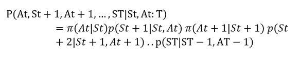
We can define the same trajectory probability in terms of important sampling as follows:

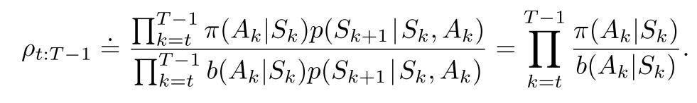
From eq. 6 it is clear that an important sampling ratio is defined as the probability of trajectory under target policy π divided by the probability of trajectory under behavior policy b. We can also infer that the transition probability terms cancel out leaving the ratio to be dependent on the two policies.

Where is this ratio used?

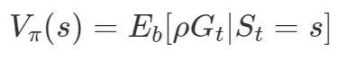
Since we are trying to estimate Vπ. We use this ratio to transform the returns obtained from behavior policy b in order to estimate the Vπ of target policy π. It is shown below :

We are now ready to define Off-policy control.

Off-policy Monte Carlo Control

Recall that our aim is to improve the target policy from the returns obtained from the behavior policy. The two policies are completely unrelated. While the target policy can be deterministic i.e. it can act greedy w.r.t. the q-function but we want our behavior policy to be exploratory. To ensure this we need to make sure we get enough returns from behavior policy about each state-action pair. The behavior policy is generally soft, meaning every state-action pair has a non-zero probability of being selected which ensures that each state-action is visited an infinite number of times.

Also, recall that using incremental means we can update/tweak our value function in the direction of optimal target policy on the go as follows :

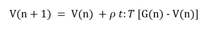
The eq. 10 shows the update rule for first n returns which is weighted by the important sampling ratio. This ratio is generally weighted important sampling ratio.

That it! Kudos on coming this far!🤖🐱‍👤

Also, I am overwhelmed by the responses on my previous RL blogs. Thank you and I hope this blog helps in the same way. Next time, we will look into Temporal-difference learning.

References:

[1] Reward M-E-M-E

[2] Richard S. Sutton, and Andy G. Barto. Reinforcement learning: An introduction.

[3] Robot M-E-M-E

[4] David Silver RL lectures

---

Reinforcement Learning: Monte-Carlo Learning was originally published in Towards AI on Medium, where people are continuing the conversation by highlighting and responding to this story.

Join thousands of data leaders on the AI newsletter. It’s free, we don’t spam, and we never share your email address. Keep up to date with the latest work in AI. From research to projects and ideas. If you are building an AI startup, an AI-related product, or a service, we invite you to consider becoming a sponsor.

Published via Towards AI