PatchTST — A Step Forward in Time Series Forecasting
Last Updated on June 28, 2023 by Editorial Team
Author(s): M. Haseeb Hassan
Originally published on Towards AI.
Gain a practical understanding of the PatchTST algorithm and its application in Python, along with N-BEATS and N-HiTS, by transitioning from theoretical knowledge to hands-on implementation.

Transformer-based models have demonstrated their effectiveness in various domains, including natural language processing (evidenced by models like BERT and GPT) and computer vision. However, in the realm of time series analysis, MLP models like N-BEATS and N-HiTS have predominantly achieved state-of-the-art performance. Recent research reveals that even simple linear models outperform complex transformer-based forecasting models across multiple benchmark datasets.
Nevertheless, a novel transformer-based model called PatchTST has emerged as a breakthrough in long-term forecasting tasks. PatchTST, short for patch time series transformer, was introduced in Nie, Nguyen et al.’s paper titled “A Time Series is Worth 64 Words: Long-Term Forecasting with Transformers,” published in March 2023. The proposed approach outperforms other transformer-based models, establishing new benchmarks for accurate long-term forecasting.
1. PatchTST
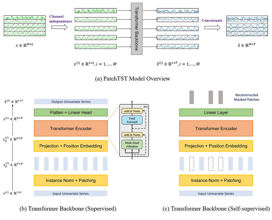
As previously mentioned, PatchTST is an acronym for patch time series transformer, indicating its utilization of patching and the transformer architecture. It incorporates channel-independence to handle multivariate time series data. The overall structure of PatchTST is depicted below.

The figure provided above contains a wealth of valuable information. It highlights the essential aspects of PatchTST, including its utilization of channel independence to predict multivariate time series. The transformer backbone of the model incorporates patching, represented by the vertical rectangles. Additionally, PatchTST offers two distinct versions: supervised and self-supervised.
Now, let’s delve deeper into the architecture and internal mechanisms of PatchTST to gain a comprehensive understanding of its functionality.
1.1 Channel Independence
In this context, a multivariate time series is treated as a multi-channel signal, where each individual time series represents a distinct channel that encapsulates a specific signal.

The provided figure illustrates the process of breaking down a multivariate time series into separate individual series. Each of these series is then utilized as an input token in the Transformer backbone. Predictions are generated independently for each series, and the outcomes are combined through concatenation to produce the final predictions.
1.2 Patching
The majority of research efforts in Transformer-based forecasting models have focused on developing novel mechanisms to simplify the original attention mechanism. However, these models still heavily rely on point-wise attention, which is not ideal for effective time series analysis.
In time series forecasting, the goal is to capture the relationships between past and future time steps in order to make accurate predictions. Point-wise attention, however, only considers information from a single time step, disregarding the contextual information surrounding it. Essentially, it isolates a specific time step and fails to take into account the broader temporal context. This is akin to trying to comprehend the meaning of a word without considering the words surrounding it within a sentence.
To address this limitation, PatchTST leverages the concept of patching to extract local semantic information within time series data. By incorporating patching, PatchTST captures meaningful patterns and dependencies within the time series, enabling a more holistic understanding of the data and facilitating accurate forecasting.
1.2.1 How Patching Works?
Each input series is divided into patches, which are simply shorter series coming from the original one.

In the PatchTST model, patches can be either overlapping or non-overlapping, offering flexibility in the design. The number of patches formed is determined by the length of the patch (P) and the stride (S). The stride, similar to convolutional operations, denotes the number of time steps that separate the starting points of consecutive patches.

The provided figure illustrates the outcome of patching. In this depiction, we observe a time series with a length of 15 time steps (L), employing a patch length of 5 (P) and a stride of 5 (S). As a result, the series is divided into three distinct patches.
1.2.2 Advantages
By implementing patching, the model can capture local semantic meaning by considering groups of time steps rather than focusing on individual time steps. Additionally, patching offers the advantage of significantly reducing the number of tokens processed by the transformer encoder. Each patch serves as an input token, leading to a reduction in token count from L to approximately L/S.
This approach effectively reduces the space and time complexity of the model, enabling the utilization of longer input sequences for extracting meaningful temporal relationships. As a result, the model becomes faster, lighter, and capable of handling extended input sequences, enhancing its potential to gain deeper insights into the time series data and generate more accurate forecasts.
1.3 Transformer Encoder
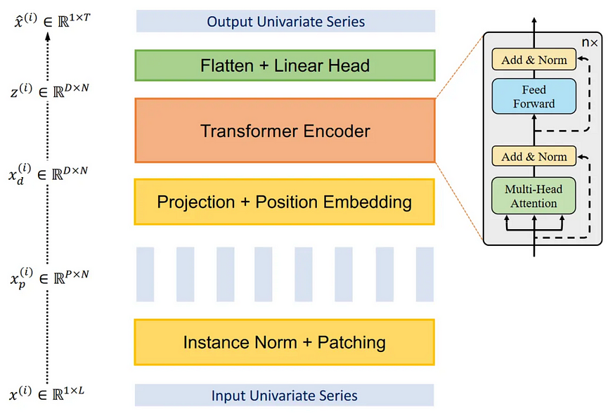
After the time series undergoes the patching process, it is subsequently passed into the transformer encoder, employing the conventional transformer architecture without any modifications. The resulting output from the transformer encoder is then fed into a linear layer, where predictions are generated based on the processed information.
1.4 Improvement through Representation Learning
The authors of the paper suggested another improvement to the model by using representation learning.

The provided figure demonstrates that PatchTST has the capability to leverage self-supervised representation learning to capture abstract representations of the data, potentially leading to improved forecasting performance.
The self-supervised learning process is straightforward: random patches within the time series are masked, indicated by the blank vertical rectangles depicted in the figure. Subsequently, the model is trained to reconstruct the original patches, illustrated at the top of the figure as the grey vertical rectangles.
Now that we have gained a comprehensive understanding of how PatchTST operates, it is time to assess its performance in comparison to other models.
2. Forecasting with PatchTST
In the mentioned research paper, PatchTST is compared to other Transformer-based models. However, recent publications have introduced MLP-based models such as N-BEATS and N-HiTS, which have also showcased exceptional performance in long-horizon forecasting tasks.
The complete source code pertaining to this section can be accessed on GitHub.
In the following analysis, we will apply PatchTST, along with N-BEATS and N-HiTS, and assess their respective performances. To conduct this evaluation, we will utilize the Exchange dataset, which is a widely adopted benchmark dataset for long-term forecasting in the research community. This dataset encompasses the daily exchange rates of eight countries in relation to the US dollar, spanning from 1990 to 2016. The availability of the dataset is governed by the MIT License.
2.1 Initial Test
To begin, we will import the necessary libraries for our analysis. Specifically, we will utilize the neuralforecast library, which offers a readily available implementation of PatchTST. Additionally, we will employ the datasetsforecastlibrary, which conveniently provides access to various well-known datasets used for evaluating forecasting algorithms.
import torch
import numpy as np
import pandas as pd
import matplotlib.pyplot as plt

from neuralforecast.core import NeuralForecast
from neuralforecast.models import NHITS, NBEATS, PatchTST

from neuralforecast.losses.pytorch import MAE
from neuralforecast.losses.numpy import mae, mse

from datasetsforecast.long_horizon import LongHorizon
If CUDA is installed on your system, neuralforecast will automatically utilize your GPU for model training. However, since I don’t have CUDA installed, I won’t be performing extensive hyperparameter tuning or training on large datasets.
2.1 Dataset
Once that step is complete, let’s proceed with downloading the Exchange dataset.
Y_df, X_df, S_df = LongHorizon.load(directory="./data", group="Exchange")
In the given code snippet, we obtain three DataFrames. The first DataFrame consists of the daily exchange rates for each country. The second DataFrame contains exogenous time series, and the third DataFrame includes static exogenous variables, such as day, month, year, hour, or any other known future information.
For the purpose of this exercise, we will focus only on the “Y_df” DataFrame.
Now, let’s visualize one of the series to get a better understanding of the data we are working with. In this case, I have chosen to plot the series for the first country (unique_id = 0), but you can choose to plot any other series of your preference.
u_id = '0'

x_plot = pd.to_datetime(Y_df[Y_df.unique_id==u_id].ds)
y_plot = Y_df[Y_df.unique_id==u_id].y.values

x_plot

x_val = x_plot[n_time - val_size - test_size]
x_test = x_plot[n_time - test_size]

fig, ax = plt.subplots(figsize=(12,8))
ax.plot(x_plot, y_plot)
ax.set_xlabel('Date')
ax.set_ylabel('Exhange rate')
ax.axvline(x_val, color='black', linestyle='--')
ax.axvline(x_test, color='black', linestyle='--')

plt.text(x_val, -2, 'Validation', fontsize=12)
plt.text(x_test,-2, 'Test', fontsize=12)

plt.tight_layout()

2.2 Model
Now that we have familiarized ourselves with the data, we can begin the modeling process using neuralforecast. Firstly, we need to define the forecasting horizon. In this case, we will use a horizon of 96-time steps, which aligns with the horizon used in the PatchTST paper.
To ensure a fair evaluation of each model, I have set the input size to be twice the horizon (192-time steps) and limited the maximum number of training epochs to 50. The remaining hyperparameters will be kept at their default values.
horizon = 96

models = [NHITS(h=horizon,
 input_size=2*horizon,
 max_steps=50),
 NBEATS(h=horizon,
 input_size=2*horizon,
 max_steps=50),
 PatchTST(h=horizon,
 input_size=2*horizon,
 max_steps=50)]
Then, we initialize the NeuralForecastobject, by specifying the models we want to use and the frequency of the forecast, which in this is case is daily.
nf = NeuralForecast(models=models, freq='D')
Now, we can make predictions.
2.3 Forecasting
To generate predictions, we utilize the cross_validationmethod, which allows us to utilize the validation and test sets. This method will provide us with a DataFrame that contains predictions from all models, along with their corresponding true values.
preds_df = nf.cross_validation(df=Y_df, val_size=val_size, test_size=test_size, n_windows=None)
In order to evaluate the models, we need to reshape the arrays of actual and predicted values. This reshaping is done to ensure that the arrays have the shape (number of series, number of windows, forecast horizon).
y_true = preds_df['y'].values
y_pred_nhits = preds_df['NHITS'].values
y_pred_nbeats = preds_df['NBEATS'].values
y_pred_patchtst = preds_df['PatchTST'].values

n_series = len(Y_df['unique_id'].unique())

y_true = y_true.reshape(n_series, -1, horizon)
y_pred_nhits = y_pred_nhits.reshape(n_series, -1, horizon)
y_pred_nbeats = y_pred_nbeats.reshape(n_series, -1, horizon)
y_pred_patchtst = y_pred_patchtst.reshape(n_series, -1, horizon)
With that done, we can optionally plot the predictions of our models. Here, we plot the predictions in the first window of the first series.
fig, ax = plt.subplots(figsize=(12,8))
ax.plot(y_true[0, 0, :], label='True')
ax.plot(y_pred_nhits[0, 0, :], label='N-HiTS', ls='--')
ax.plot(y_pred_nbeats[0, 0, :], label='N-BEATS', ls=':')
ax.plot(y_pred_patchtst[0, 0, :], label='PatchTST', ls='-.')
ax.set_ylabel('Exchange rate')
ax.set_xlabel('Forecast horizon')
ax.legend(loc='best')
plt.tight_layout()

The visualization of the predictions in this figure appears to be disappointing, as N-BEATS and N-HiTS models show predictions that significantly deviate from the actual values. On the other hand, PatchTST’s predictions, although not perfect, appear to be relatively closer to the actual values. However, it’s important to note that this assessment is based on the visualization of predictions for just one series and within a single prediction window. Thus, it should be interpreted cautiously and further analysis is needed to make conclusive judgments.
2.4 Evaluation
Now, we will proceed with evaluating the performance of each model. In line with the methodology outlined in the paper, we will utilize two commonly used performance metrics: Mean Absolute Error (MAE) and Mean Squared Error (MSE).

From the presented table, it is evident that PatchTST emerges as the top-performing model, achieving the lowest values for both MAE and MSE metrics. It is important to note that this experiment is not exhaustive, as it solely focuses on one dataset and one specific forecast horizon. Nevertheless, the results are intriguing, showcasing the competitive capabilities of a Transformer-based model compared to the state-of-the-art MLP models.
3. Conclusion
PatchTST, a Transformer-based model, incorporates patching to extract localized semantic meaning in time series data. This approach enables faster training and the ability to handle longer input windows. Notably, PatchTST has demonstrated state-of-the-art performance compared to other Transformer-based models.
In our experiment, we observed its superior performance in comparison to N-BEATS and N-HiTS. While this does not imply that PatchTST is universally superior to N-HiTS or N-BEATS, it presents an intriguing option for long-horizon forecasting tasks. Thank you for reading! I hope you found this information enjoyable and informative.
References
A Time Series is Worth 64 Words: Long-Term Forecasting with Transformersby Nie Y., Nguyen N. et al.
Neuralforecast by Olivares K., Challu C., Garza F., Canseco M., Dubrawski A.
If you enjoyed the article and wish to show your support, make sure to:
- U+1F44F Give a round of applause (50 claps) to help get featured
- U+1F465 Follow me on Medium to stay updated with my latest content
- U+1F4F0 Explore more articles on my Medium Profile
- U+1F514 Connect with me on LinkedIn, Twitter, and GitHub
Join thousands of data leaders on the AI newsletter. Join over 80,000 subscribers and keep up to date with the latest developments in AI. From research to projects and ideas. If you are building an AI startup, an AI-related product, or a service, we invite you to consider becoming a sponsor.
Published via Towards AI
Towards AI Academy
We Build Enterprise-Grade AI. We'll Teach You to Master It Too.
15 engineers. 100,000+ students. Towards AI Academy teaches what actually survives production.
Start free — no commitment:
→ 6-Day Agentic AI Engineering Email Guide — one practical lesson per day
→ Agents Architecture Cheatsheet — 3 years of architecture decisions in 6 pages
Our courses:
→ AI Engineering Certification — 90+ lessons from project selection to deployed product. The most comprehensive practical LLM course out there.
→ Agent Engineering Course — Hands on with production agent architectures, memory, routing, and eval frameworks — built from real enterprise engagements.
→ AI for Work — Understand, evaluate, and apply AI for complex work tasks.
Note: Article content contains the views of the contributing authors and not Towards AI.


