Logistic Regression’s Journey with Imbalanced Data

Author(s): Anand Raj

Originally published on Towards AI.

Visual intuition behind the effect of imbalanced data on logistic regression

In the vast landscape of data-driven decision-making, class imbalance is a subtle yet influential factor that can significantly impact the performance of machine learning models. Class imbalance occurs when the distribution of instances across different classes in a dataset is uneven, with one class vastly outnumbering the others. This scenario is prevalent in various real-world applications, from medical diagnoses to fraud detection and sentiment analysis.

In the presence of class imbalance, models may exhibit a bias towards the majority class, leading to suboptimal performance on the minority class. The consequences of misclassification can be severe, primarily when the minority class represents critical or rare events. Understanding how to navigate the complexities introduced by imbalanced classes is crucial for building robust and reliable machine-learning models.

How does class imbalance occur?

There are many different sources of imbalanced datasets, and each one poses different difficulties for machine learning applications. The inherent class distribution captures instances in which imbalances arise from the classes’ inherent predominance in real-world circumstances. Positive cases may be far more rare than negative ones, for example, in fraud detection or rare disease diagnosis. When data collection procedures are intrinsically biased, such as when samples are drawn from particular demographics or geographic areas, imbalances are introduced via sampling bias. Mislabeled cases or missing data are examples of data collection problems that can lead to skewed class distributions. Some classes may be underrepresented in the dataset because of the expense and work involved in gathering data for them.

Common domains where imbalance occurs:

• Fraud Detection.
• Claim Prediction
• Default Prediction.
• Churn Prediction.
• Spam Detection.
• Anomaly Detection.
• Outlier Detection.
• Intrusion Detection
• Conversion Prediction.

We will explore an instance where the imbalance in data increases, observing its impact on the decision surface.

I have used the iris dataset from Kaggle and tweaked it a little as per our needs.

Let’s Consider these five scenarios:

Scenario 1: Balanced Dataset (n​Versicolor : nVirginica ≈ 1:1​)
Scenario 2: Imbalanced Dataset (n​Versicolor : nVirginica ≈ 1:2)
Scenario 3: Imbalanced Dataset (n​Versicolor : nVirginica ≈ 1:3)
Scenario 4: Imbalanced Dataset (n​Versicolor : nVirginica​ ≈ 1:4)
Scenario 5: Imbalanced Dataset (n​Versicolor : nVirginica ≈ 1:11)

Scenario 1: “Harmony in Equilibrium”
(Balanced Dataset with n​Versicolor : nVirginica ≈ 1:1​)
An equal number of observations in Class Iris-Versicolor ≈ Class Iris-Virginica, creating a balanced symphony.

As we can see in the above image the decision surface linearly separates both classes quite well and this is because the proportions of data points in both the classes are equal.

Scenario 2: “The Delicate Imbalance ”
(Imbalanced Dataset with n​Versicolor : nVirginica ≈ 1:2​)
The count of observations in Class Iris-Versicolor is approximately half of the count in Class Iris-Virginica, revealing an uneven distribution.

With a data point proportion of 1:2, noticeable misclassifications occur among some Iris-Versicolor instances. Contrasting this with the balanced dataset (Scenario 1), the decision surface undergoes alterations, leading to less effective linear separation of the classes.

Scenario 3: “The Tipping Scales”
(Imbalanced Dataset with n​Versicolor : nVirginica ≈ 1:3​)
The count of observations in Class Iris-Versicolor is approximately one-third of the count in Class Iris-Virginica, showcasing a significant imbalance in the data distribution.

With a data point proportion of 1:3, a substantial number of misclassifications emerge, affecting nearly half of the Iris-Versicolor instances. Comparing this with the previous imbalanced dataset (Scenario 2), the performance of the decision surface degrades further. The dominance of Class Iris-Virginica plays a key role, influencing the decision surface adversely.

Scenario 4: “The Unsettling Disparity”
(Imbalanced Dataset with n​Versicolor : nVirginica ≈ 1:4​)
The count of observations in Class Iris-Versicolor is approximately one-fourth of the count in Class Iris-Virginica, illustrating a pronounced imbalance in the dataset.

With a data point proportion of 1:4, only a single data point in Class Iris-Versicolor is correctly classified, highlighting a severe imbalance. Comparing this with the preceding imbalanced dataset (Scenario 3), the performance of the decision surface further deteriorates. The overwhelming majority of data points in Class Iris-Virginica exerts significant influence, exacerbating the challenges in classification.

Scenario 5: “The Extreme Odds”
(Highly Imbalanced Dataset with n​Versicolor : nVirginica ≈ 1:11​)
The count of observations in Class Iris-Versicolor is approximately one-eleventh of the count in Class Iris-Virginica, indicating an exceptionally skewed distribution.

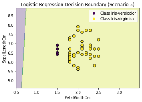
With a data point proportion of 1:11, every data point in the minority class faces misclassification. Contrasting this with the previous imbalanced dataset (Scenario 4), the performance of the decision surface experiences a significant decline. The substantial majority of data points belonging to Class Iris-Virginica exert a profound influence, leading to increased challenges in accurate classification.

Why does this happen? [Let’s do the Math]

This happens because logistic regression tries to find the best hyperplane that maximizes the distance of every data point to the optimal hyperplane (a.k.a Decision Surface). This is also called “Optimization”. The equation is as follows:

Let’s take three cases as an example.

Case 1: Both the classes are classified correctly with the Grey line as Decision Surface in the picture below.

Let’s assume we had a decision surface (The grey line represents the decision surface) that linearly separated both the classes perfectly, and the distance between the classes was 0.6 from the decision surface. The value of yi will be 1 for all the data points, as all the points are correctly classified if the black line is our decision surface.

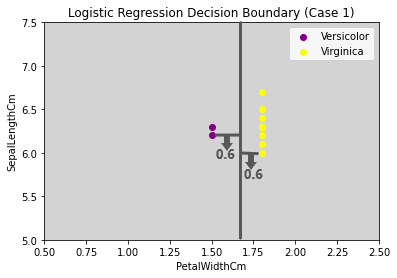
Number of data points in Versicolor = 2
Number of data points in Virginica = 7

W(Transpose) * x = 0.6 {∀ Data points}
yi = 1 {All data points are correctly classified}

Let’s compute the value the below equation will return for this scenario.

∀ Data points in Virginica = 2*Σ (1*0.6) = 1.2
∀ Data points in Versicolor = 7*Σ (1*0.6) = 4.2
∀ Data points in Versicolor and Virginica = 1.2 + 4.2 = 5.4

Case 2: Only one classified correctly (Virginica class) with the Grey line as Decision Surface in the picture below.

Let’s assume that the distance of both the classes is 1 (Sigmoid will limit any distance value above 1 to 1) from the decision surface. The value of yi will be 1 for all the Virginica data points (All Virginica data points are classified correctly), and yi will be -1 for all the Versicolor data points (All Virginica data points are classified incorrectly).

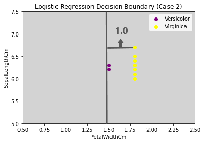
Number of data points in Versicolor = 2
Number of data points in Virginica = 7

Transpose(W) * x = 1 (∀ Data points)
yi = 1 ∀ Versicolor data points (classified correctly)
yi = -1 ∀ Virginica data points (classified incorrectly)

Let’s compute the value the below equation will return for this scenario.

∀ Data points in Virginica = 7*Σ (1*1) = 7
∀ Data points in Versicolor = 2*Σ (-1*0) = 0
∀ Data points in Versicolor and Virginica = 7 + 0= 7

Now, the agrmax function will take the highest value possible, which is 7 (Case 2).

The corresponding W* (Optimal Decision Surface will be the one in Case 2), but we know it is not the optimal decision surface. This happens due to the imbalance in the classes and the majority class dominating the minority class.

Case 3: Let’s take a scenario where the data is balanced.

Let’s assume we had a decision surface (The grey line represents the decision surface) that linearly separated both the classes perfectly and the distance between the classes was 0.6 from the decision surface. The value of yi will be 1 for all the data points, as all the points are correctly classified if the black line is our decision surface.

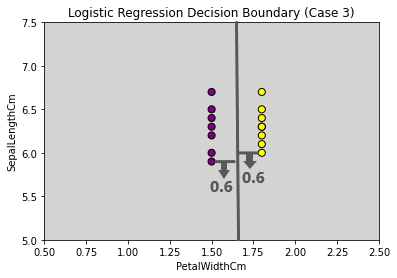
Number of data points in Versicolor = 7
Number of data points in Virginica = 7

W(Transpose) * x = 0.6 {∀ Data points}
yi = 1 {All data points are correctly classified}

Let’s compute the value the below equation will return for this scenario.

∀ Data points in Virginica = 7*Σ (1*0.6) = 4.2
∀ Data points in Versicolor = 7*Σ (1*0.6) = 4.2
∀ Data points in Versicolor and Virginica = 4.2 + 4.2 = 8.4

Now, the agrmax function will take the highest value possible, which is 8.4 (Case 3). Therefore, it chooses the right decision surface, as shown in case 3.

The below representation is what the Logistic Regression in scikit-learn returns.

We saw that imbalanced data could influence the decision surface, resulting in the model’s lousy performance. Therefore, it’s essential to handle this imbalance in the data, which can be done in the following ways.

1.Resampling techniques
2. Data augmentation
3. Synthetic minority over-sampling technique (SMOTE)
4. Ensemble techniques
5. One-class classification
6. Cost-sensitive learning
7. Evaluation metrics for imbalanced data

These are just few ways there could be many more so keep exploring.

Here is the link to the code on my GitHub.

Hope you liked the article!!!!

You may reach out to me on LinkedIn.

https://www.linkedin.com/in/anand-raj-4334a91b3/

Join thousands of data leaders on the AI newsletter. Join over 80,000 subscribers and keep up to date with the latest developments in AI. From research to projects and ideas. If you are building an AI startup, an AI-related product, or a service, we invite you to consider becoming a sponsor.

Published via Towards AI