Introduction to Audio Machine Learning

Author(s): Sujay Kapadnis

Originally published on Towards AI.

I am currently developing an Audio Speech Recognition system, so I needed to brush up my knowledge on the basics regarding it. This article is the result of that.

Introduction to Audio

Index

1. Introduction

Sound —

• Sound is a continuous signal and has infinite signal values
• Digital devices require finite arrays and thus, we need to convert them into a series of discrete values
• AKA Digital Representation
• Sound Power — Rate at which energy is transferred(Watt)
• Sound Intensity — Sound Power per unit area(Watt/m**2)

Audio File formats —

1. .wav
2. .flac(free lossless audio codec)
3. .mp3

Files formats are differentiated by the way they compress digital representation of the audio signal

Steps of conversion —

• The microphone captures an analog signal.
• The soundwave is then converted into an electrical signal.
• this electrical signal is then digitized by an analog-to-digital converter.

Sampling

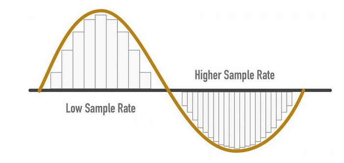
• It is the process of measuring the value of a signal at fixed time steps
• Once sampled, the sampled waveform is in a discrete format

Sampling rate/ Sampling frequency

• No. of samples taken per second
• e.g. if 1000 samples are taken per second, then sampling rate(SR) = 1000
• HIGHER SR -> BETTER AUDIO QUALITY

SR considerations

• Sampling Rate = (Highest frequency that can be captured from a signal) * 2
• For the Human ear- the audible frequency is 8KHz hence we can say that the Sampling rate(SR) is 16KHz
• Although more SR gives better audio quality does not mean we should keep increasing it.
• After the required line it does not add any information and only increases the computation cost
• Also, low SR can cause a loss of information

Points to remember —

• While training all audio samples to have the same sampling rate
• If you are using a pre-trained model, the audio sample should be resampled to match the SR of the audio data model trained on
• If Data from different SRs is used, then the model does not generalize well

Amplitude —

• Sound is made by a change in air pressure at human audible frequencies
• Amplitude — sound pressure level at that instant measured in dB(decibel)
• Amplitude is a measure of loudness

Bit Depth —

• Describes how much precision value can be described
• The higher the bit depth, the more closely the digital representation resembles the original continuous sound wave
• Common values of bit depth are 16-bit and 24-bit

Quantizing —

Initially, audio is in continuous form, which is a smooth wave. To store it digitally, we need to store it in small steps; we perform quantizing to do that.

You can say that Bit Depth is the number of steps needed to represent audio

• 16-bit audio needs — 65536 steps
• 24-bit audio need — 16777216 steps
• This quantizing induces noise, hence high bit depth is preferred
• Although this noise is not a problem
• 16 and 24-bit audio are stored in int samples whereas 32-bit audio samples are stored in floating points
• The model required a floating point, so we need to convert this audio into a floating point before we train the model

Implementation —

#load the library
import librosa

#librosa.load function returns the audio array and sampling rate
audio, sampling_rate = librosa.load(librosa.ex('pistachio'))

import matplotlib.pyplot as plt
plt.figure().set_figwidth(12)
librosa.display.waveshow(audio,sr = sampling_rate)

• amplitude was plotted on the y-axis and time on the x-axis
• ranges from [-1.0,1.0] — already a floating point number

print(len(audio))
print(sampling_rate/1e3)
>>1560384
>>22.05

## Frequency Spectrum
import numpy as np
# rather than focusing on each discrete value lets just see first 4096 values
input_data = audio[:4096]


# DFT = discrete fourier transform
# this frequency spectrum is plotted using DFT
window = np.hanning(len(input_data))
window

>>array([0.00000000e+00, 5.88561497e-07, 2.35424460e-06, ...,
 2.35424460e-06, 5.88561497e-07, 0.00000000e+00])

dft_input = input_data * window

figure = plt.figure(figsize = (15,5))
plt.subplot(131)
plt.plot(input_data)
plt.title('input')
plt.subplot(132)
plt.plot(window)
plt.title('hanning window')
plt.subplot(133)
plt.plot(dft_input)
plt.title('dft_input')
# similar plot is generated for every instance

Discrete Frequency Transform = DFT

• Would you agree with me if I were to say that up until we have discrete signal data?
• If you do, then you can understand that up until now, we had the data in the time domain, and now we want to convert it into the frequency domain. That’s why sir DFT is here to help

# calculate the dft - discrete fourier transform
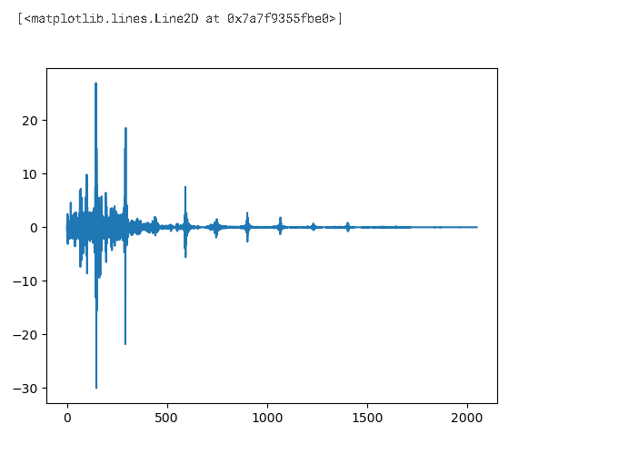
dft = np.fft.rfft(dft_input)
plt.plot(dft)

# amplitude 
amplitude = np.abs(dft)
# convert it into dB
amplitude_dB = librosa.amplitude_to_db(amplitude,ref = np.max)

# sometimes people want to use power spectrum -> A**2

Why take the absolute?

When we took amplitude, we applied the abs function, the reason being the complex number

• the output returned after the Fourier transform is in complex form, and taking absolute gave us the magnitude, thus absolute.

print(len(amplitude))
print(len(dft_input))
print(len(dft))
>>2049
>>4096
>>2049

Why’s the updated array (half+1) of the original array?

When the DFT is computed for purely real input, the output is Hermitian-symmetric, i.e., the negative frequency terms are just the complex conjugates of the corresponding positive-frequency terms, and the negative-frequency terms are therefore redundant. This function does not compute the negative frequency terms, and the length of the transformed axis of the output is therefore n//2 + 1. [source – documentation]

# frequency
frequency = librosa.fft_frequencies(n_fft=len(input_data),sr = sampling_rate)

plt.figure().set_figwidth(12)
plt.plot(frequency, amplitude_dB)
plt.xlabel("Frequency (Hz)")
plt.ylabel("Amplitude (dB)")
plt.xscale("log")

• As mentioned earlier, time domain -> frequency domain
• The frequency domain is usually plotted on a logarithmic scale

Spectrograms —

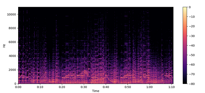
• shows how the frequency changes w.r.t. time
• The algorithm that performs this transformation is soft = short time-frequency transform

How to create a spectrogram —

• spectrograms are a stack of frequency transforms, how? let us see
• For given audio, we take small segments and find their frequency spectrum. After that, we just stack them along the time axis. The resultant diagram is a spectrogram
• librosa.stft by default splits into 2048 segments

Frequency Spectrum —

• Represents the amplitude of different frequencies at a single moment in time.
• The frequency spectrum is more suitable for understanding the frequency components present in a signal at a specific instant. Both representations are valuable tools for understanding the characteristics of signals in the frequency domain.
• AMPLITUDE vs. FREQUENCY

Spectrogram —

• Represents the changes in frequency content over time by breaking the signal into segments and plotting their frequency spectra over time.
• The spectrogram is particularly useful for analyzing and visualizing time-varying signals, such as audio signals or time-series data, as it provides insights into how the frequency components evolve over different time intervals.
• FREQUENCY vs. TIME

spectogram = librosa.stft(audio)
spectogram_to_dB = librosa.amplitude_to_db(np.abs(spectogram),ref = np.max)

plt.figure().set_figwidth(12)
librosa.display.specshow(spectogram_to_dB, x_axis="time", y_axis="hz")
plt.colorbar()

Mel Spectrograms —

• The spectrogram on different frequency scales.

Before proceeding, one must remember that.

• At lower frequencies, humans are more sensitive to audio changes than at higher frequencies
• This sensitivity changes logarithmically with an increase in frequency
• So in simpler terms, a mel spectrogram is a compressed version of the spectrogram.

MelSpectogram = librosa.feature.melspectrogram(y=audio, sr=sampling_rate, n_mels=128, fmax=8000)
MelSpectogram_dB = librosa.power_to_db(MelSpectogram, ref=np.max)

plt.figure().set_figwidth(12)
librosa.display.specshow(MelSpectogram_dB, x_axis="time", y_axis="mel", sr=sampling_rate, fmax=8000)
plt.colorbar()

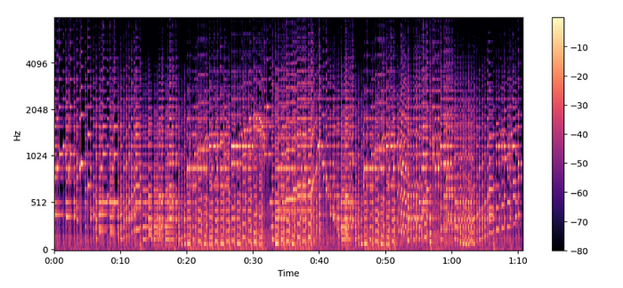
• The above example is used librosa.power_to_db() as librosa.feature.melspectrogram() is used to create a power spectrogram.

Conclusion —

Mel Spectogram helps capture more meaningful features than normal spectrogram and hence is popular.

Reference —

Huggingface

Personal Kaggle Kernel (for your practice)

Socials —

LinkedIn

Kaggle

If you liked the article, don’t forget to show appreciation by clapping. See You in the next notebook, where we’ll see ‘How to load and stream the audio data.’

Join thousands of data leaders on the AI newsletter. Join over 80,000 subscribers and keep up to date with the latest developments in AI. From research to projects and ideas. If you are building an AI startup, an AI-related product, or a service, we invite you to consider becoming a sponsor.

Published via Towards AI