Graphs in Motion: Spatio-Temporal Dynamics with Graph Neural Networks

Author(s): Najib Sharifi

Originally published on Towards AI.

Interconnected graphical data is all around us, ranging from molecular structures to social networks and design structures of cities. Graph Neural Networks (GNNs) are emerging as a powerful method of modeling and learning the spatial and graphical structure of such data. It has been applied to protein structures and other molecular applications such as drug discovery as well as modelling systems such as social networks. Recently, the standard GNN has been combined with ideas from other ML models to develop exciting, innovative applications. One such development is the integration of GNN with sequential models — Spatio-Temporal GNN that is able to capture both the temporal and spatial (hence the name) dependences of data.

GNNs is a relatively young field with a lot of potential because most of ‘man-made’ systems in the world are graphical structure in nature for example the internet is a essentially one very large graph, molecular structure, chemical plants, structure of cities etc can all be represented as graphs. Advances in GNNs could be the next big field of AI.

GNN models and sequential models (such as simple RNNs, LSTM or GRU) are complex in their own right. Combining these models for both spatial and temporal dependence is powerful, but difficult. Difficult to understand and difficult to implement. In this article, we’ll dive deep into the principles behind these models and also implement a relatively simple example of such a model to unlock a deeper comprehension of their capabilities and applications.

Graph Neural Network (GNN)

I will provide a short discussion on GNNs here. A graph G can be defined as G = (V, E), where V is the set of nodes, and E are the edges between them.

The feature matrix of a graph containing n nodes and each with f features, is the concatenation all the features:

The key property of GNNs is the message passing between all connected nodes, this neighbour feature transformation and aggregation is written as:

Where A is the Adjacency matrix of the graph, I is the identity matrix allowing for self-connection. Although this is not the complete equation, this is basis of graph convolution network that can learn the spatial dependence between different nodes. I have explained this in more detail in my previous article. An illustration of GNN:

Spatio-Temporal Graph Neural Network

The concept behind ST-GNN is illustrated in Figure 2, where each time step is a graph and is passed through a GCN/GAT network to obtain the resultant encoded graph that embed the inter-relational spatial dependence. Subsequently, these encoded graphs can be modelled exactly like time series data as long as the integrity of the graphical structure of the data at each time step is preserved. Figure 2 demonstrates these two steps, the temporal model could be any sequential model ranging from ARIMA or simple recurrent neural network to transformers.

For a simple Recurrent Neural Network, the temporal model is illustrated in Figure 3. In the demonstration that follows, we’ll use a Gated Recurrent Unit (GRU).

This is the principle behind ST-GNN; a combination of GNNs and sequential models such as RNN, LSTM, GRU, Transformers etc. If you are already familiar with with these sequential and GNNs models then this is probably fairly straight forward.

Implementing ST-GNNs With Pytorch

Due to limited non-proprietary data that is simple enough for demonstrations purposes, I will use stock market data of large tech companies. Whilst this data is inherently not graphical data in nature, this kind of network could potentially capture the inter-dependence of these companies e.g. the performance of one company (good or bad) might in turn impact the value of other companies in the market. But this is only a demonstration, I am not actually advocating for ST-GNN in stock market prediction.

Dataset Download & Scale

import yfinance as yf
import datetime as dt
import pandas as pd
from sklearn.preprocessing import StandardScaler

import plotly.graph_objs as go
from plotly.offline import iplot
import matplotlib.pyplot as plt

############ Dataset download #################
start_date = dt.datetime(2013,1,1)
end_date = dt.datetime(2024,3,7)
#loading from yahoo finance
google = yf.download("GOOGL",start_date, end_date)
apple = yf.download("AAPL",start_date, end_date)
Microsoft = yf.download("MSFT", start_date, end_date)
Amazon = yf.download("AMZN", start_date, end_date)
meta = yf.download("META", start_date, end_date)
Nvidia = yf.download("NVDA", start_date, end_date)
data = pd.DataFrame({'google': google['Open'],'microsoft': Microsoft['Open'],'amazon': Amazon['Open'],
 'Nvidia': Nvidia['Open'],'meta': meta['Open'], 'apple': apple['Open']})
############## Scaling data ######################
scaler = StandardScaler()
data_scaled = pd.DataFrame(scaler.fit_transform(data), columns=data.columns)

Graphical Data Transformation

Transforming the scalar time series dataset into graphical data structure. The function AdjacencyMatrix defines the adjacency matrix (connectivity) of the graph, this is usually done based on the structure of the physical systems at hand, however, I have just used a matrix of ones i.e. all nodes are connected to all other nodes here.

The StockMarketDataset class is designed to create the datasets for training ST-GNNs. The DatasetCreate method generates sequences of data. The _create_edges method constructs the edges of the graph using the adjacency matrix. The _create_sequences method generates sequences of data by sliding the window over the input stock market data. This data preparation code could very easily be adapted for other problems

def AdjacencyMatrix(L):
 AdjM = np.ones((L,L))
 return AdjM

class StockMarketDataset:
 def __init__(self, W,N_hist, N_pred):
 self.W = W
 self.N_hist = N_hist
 self.N_pred = N_pred
 def DatasetCreate(self):
 num_days, self.n_node = data_scaled.shape
 n_window = self.N_hist + self.N_pred
 edge_index, edge_attr = self._create_edges(self.n_node)
 sequences = self._create_sequences(data_scaled, self.n_node, n_window, edge_index, edge_attr)
 return sequences
 def _create_edges(self, n_node):
 edge_index = torch.zeros((2, n_node**2), dtype=torch.long)
 edge_attr = torch.zeros((n_node**2, 1))
 num_edges = 0
 for i in range(n_node):
 for j in range(n_node):
 if self.W[i, j] != 0:
 edge_index[:, num_edges] = torch.tensor([i, j], dtype=torch.long)
 edge_attr[num_edges, 0] = self.W[i, j]
 num_edges += 1
 edge_index = edge_index[:, :num_edges]
 edge_attr = edge_attr[:num_edges]
 return edge_index, edge_attr
 def _create_sequences(self, data, n_node, n_window, edge_index, edge_attr):
 sequences = []
 num_days, _ = data.shape
 for i in range(num_days):
 sta = i
 end = i+n_window
 full_window = np.swapaxes(data[sta:end, :], 0, 1)
 g = Data(x=torch.FloatTensor(full_window[:, :self.N_hist]),
 y=torch.FloatTensor(full_window[:, self.N_hist:]),
 edge_index=edge_index,
 num_nodes=n_node)
 sequences.append(g)
 return sequences

Train-Test Split

The code below essentially uses a custom function to do Train-Validation-Test split. The data is shuffled (through their indices) to ensure the graphical structure of data is preserved. This ensures, the training is obtained over the while series rather than just the first 80%.

from torch_geometric.loader import DataLoader

def train_val_test_splits(sequences, splits):
 total = len(sequences)
 split_train, split_val, split_test = splits 
 
 # Calculate split indices
 idx_train = int(total * split_train)
 idx_val = int(total * (split_train + split_val))
 indices = [i for i in range(len(sequences)-100)]
 random.shuffle(indices)
 train = [sequences[index] for index in indices[:idx_train]]
 val = [sequences[index] for index in indices[idx_train:idx_val]]
 test = [sequences[index] for index in indices[idx_val:]]
 return train, val, test
'''Setting up the hyper paramaters'''
n_nodes = 6
n_hist = 50
n_pred = 10
batch_size = 32
# Adjacency matrix 
W = AdjacencyMatrix(n_nodes)
# transorm data into graphical time series 
dataset = StockMarketDataset(W, n_hist, n_pred)
sequences = dataset.DatasetCreate() 
# train, validation, test split
splits = (0.9, 0.05, 0.05) 
train, val, test = train_val_test_splits(sequences, splits)
train_dataloader = DataLoader(train, batch_size=batch_size, shuffle=True, drop_last = True)
val_dataloader = DataLoader(val, batch_size=batch_size, shuffle=True, drop_last=True)
test_dataloader = DataLoader(test, batch_size=batch_size, shuffle=True, drop_last = True)

Model Definition

The model definition within Pytorch include a GATConv and 2 GRU layers as encoders and 1 GRU layer + fully connected layer as the decoder. The GATconv is the GNN part that aim to capture the spatial dependence and the GRU layers aim to capture the temporal dynamics of the data. The code include a lot of data reshaping to be in line with what each layer expects. You should print the shape of x at different stages in the forward pass to check the dimensions and compare this against the documentation for expected input dimensions into GRU and Linear layers.

import torch
import torch.nn.functional as F
from torch_geometric.nn import GATConv

class ST_GNN_Model(torch.nn.Module):
 def __init__(self, in_channels, out_channels, n_nodes,gru_hs_l1, gru_hs_l2, heads=1, dropout=0.01):
 super(ST_GAT, self).__init__()
 self.n_pred = out_channels
 self.heads = heads
 self.dropout = dropout
 self.n_nodes = n_nodes
 self.gru_hidden_size_l1 = gru_hs_l1
 self.gru_hidden_size_l2 = gru_hs_l2
 self.decoder_hidden_size = self.gru_hidden_size_l2
 # enconder GRU layers
 self.gat = GATConv(in_channels=in_channels, out_channels=in_channels, 
 heads=heads, dropout=dropout, concat=False)
 self.encoder_gru_l1 = torch.nn.GRU(input_size=self.n_nodes, 
 hidden_size=self.gru_hidden_size_l1, num_layers=1,
 bias = True)
 self.encoder_gru_l2 = torch.nn.GRU(input_size=self.gru_hidden_size_l1,
 hidden_size=self.gru_hidden_size_l2, num_layers = 1,
 bias = True)
 self.GRU_decoder = torch.nn.GRU(input_size = self.gru_hidden_size_l2, hidden_size = self.decoder_hidden_size,
 num_layers =1, bias = True, dropout= self.dropout)
 
 self.prediction_layer = torch.nn.Linear(self.decoder_hidden_size, self.n_nodes*self.n_pred, bias= True) 

 def forward(self, data, device):
 x, edge_index = data.x, data.edge_index
 if device == 'cpu':
 x = torch.FloatTensor(x)
 else:
 x = torch.cuda.FloatTensor(x)
 x = self.gat(x, edge_index)
 x = F.dropout(x, self.dropout, training=self.training)
 batch_size = data.num_graphs
 n_node = int(data.num_nodes / batch_size)
 x = torch.reshape(x, (batch_size, n_node, data.num_features))
 x = torch.movedim(x, 2, 0)
 encoderl1_outputs, _ = self.encoder_gru_l1(x)
 x = F.relu(encoderl1_outputs)
 encoderl2_outputs, h2 = self.encoder_gru_l2(x)
 x = F.relu(encoderl2_outputs)
 x, _ = self.GRU_decoder(x,h2)
 x = torch.squeeze(x[-1,:,:])
 x = self.prediction_layer(x)
 x = torch.reshape(x, (batch_size, self.n_nodes, self.n_pred))
 x = torch.reshape(x, (batch_size*self.n_nodes, self.n_pred))
 return x

Training

The training process of ST-GNNs are pretty much the same as any network training in pytorch.

import torch
import torch.optim as optim


# Hyperparameters
gru_hs_l1 = 16
gru_hs_l2 = 16
learning_rate = 1e-3
Epochs = 50
device = 'cuda' if torch.cuda.is_available() else 'cpu'
model = ST_GNN_Model(in_channels=n_hist, out_channels=n_pred, n_nodes=n_nodes, gru_hs_l1=gru_hs_l1, gru_hs_l2 = gru_hs_l2)
pretrained = False
model_path = "ST_GNN_Model.pth"
if pretrained:
 model.load_state_dict(torch.load(model_path))
optimizer = optim.Adam(model.parameters(), lr=learning_rate, weight_decay=1e-7)
criterion = torch.nn.MSELoss()
model.to(device)
for epoch in range(Epochs):
 model.train()
 for _, batch in enumerate(tqdm(train_dataloader, desc=f"Epoch {epoch}")):
 batch = batch.to(device)
 optimizer.zero_grad()
 y_pred = torch.squeeze(model(batch, device))
 loss= criterion(y_pred.float(), torch.squeeze(batch.y).float())
 loss.backward()
 optimizer.step()
 print(f"Loss: {loss:.7f}")

Model Evaluation and Visualisation

Now that our model training is complete, let’s visualise the prediction ability of the model. The code below, for each data input, predicts the model output and subsequently plots model output vs ground truth values. The function allows results for one particular node and at a single prediction step to be extracted.

@torch.no_grad()
def Extract_results(model, device, dataloader, type=''):
 model.eval()
 model.to(device)
 n = 0
 # Evaluate model on all data
 for i, batch in enumerate(dataloader):
 batch = batch.to(device)
 if batch.x.shape[0] == 1:
 pass
 else:
 with torch.no_grad():
 pred = model(batch, device)
 truth = batch.y.view(pred.shape)
 if i == 0:
 y_pred = torch.zeros(len(dataloader), pred.shape[0], pred.shape[1])
 y_truth = torch.zeros(len(dataloader), pred.shape[0], pred.shape[1])
 y_pred[i, :pred.shape[0], :] = pred
 y_truth[i, :pred.shape[0], :] = truth
 n += 1
 y_pred_flat = torch.reshape(y_pred, (len(dataloader),batch_size,n_nodes,n_pred))
 y_truth_flat = torch.reshape(y_truth,(len(dataloader),batch_size,n_nodes,n_pred))
 return y_pred_flat, y_truth_flat

def plot_results(predictions,actual, step, node):
 predictions = torch.tensor(predictions[:,:,node,step]).squeeze()
 actual = torch.tensor(actual[:,:,node,step]).squeeze()
 pred_values_float = torch.reshape(predictions,(-1,))
 actual_values_float = torch.reshape(actual, (-1,))
 scatter_trace = go.Scatter(
 x=actual_values_float,
 y=pred_values_float,
 mode='markers',
 marker=dict(
 size=10,
 opacity=0.5, 
 color='rgba(255,255,255,0)', 
 line=dict(
 width=2,
 color='rgba(152, 0, 0, .8)', 
 )
 ),
 name='Actual vs Predicted'
 )
 line_trace = go.Scatter(
 x=[min(actual_values_float), max(actual_values_float)],
 y=[min(actual_values_float), max(actual_values_float)],
 mode='lines',
 marker=dict(color='blue'),
 name='Perfect Prediction'
 )
 data = [scatter_trace, line_trace]
 layout = dict(
 title='Actual vs Predicted Values',
 xaxis=dict(title='Actual Values'),
 yaxis=dict(title='Predicted Values'),
 autosize=False,
 width=800,
 height=600
 )
 fig = dict(data=data, layout=layout)
 iplot(fig)
y_pred, y_truth = Extract_results(model, device, test_dataloader, 'Test')
plot_results(y_pred, y_truth,9,0) # timestep, node

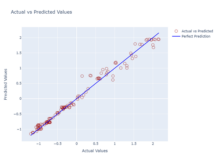
For 6 nodes (companies), given the past 50 values, 10 predictions are made. Below is a plot of 10th step prediction of the first node against ground truth. It is not bad but does not necessarily indicate good prediction. For time series data, the best estimator for the next value is always the previous one. If not trained well, these models can output values similar to the last value of input data rather than capturing the temporal dynamics.

Plot the patterns

For a given node, the function below will plot the historical input, the predictions and the ground truth to see if the prediction captures the pattern. Some examples of the forecast are presented.

@torch.no_grad()
def forecastModel(model, device, dataloader, node):
 model.eval()
 model.to(device)
 for i, batch in enumerate(dataloader):
 batch = batch.to(device)
 with torch.no_grad():
 pred = model(batch, device)
 truth = batch.y.view(pred.shape)
 # the shape should [batch_size, nodes, number of predictions]
 truth = torch.reshape(truth, [batch_size, n_nodes,n_pred])
 pred = torch.reshape(pred, [batch_size, n_nodes,n_pred])
 x = batch.x
 x = torch.reshape(x, [batch_size, n_nodes,n_hist])
 
 y_pred = torch.squeeze(pred[0, node, :])
 y_truth = torch.squeeze(truth[0,node,:])
 y_past = torch.squeeze(x[0, node, :])
 t_range = [t for t in range(len(y_past))]
 break
 t_shifted = [t_range[-1]+1+t for t in range(len(y_pred))]
 trace1 = go.Scatter(x =t_range, y= y_past, mode = "markers", name = "Historical data")
 trace2 = go.Scatter(x=t_shifted, y=y_pred, mode = "markers", name = "pred")
 trace3 = go.Scatter(x=t_shifted, y=y_truth, mode = "markers", name = "truth")
 layout = go.Layout(title = "forecasting", xaxis=dict(title = 'time'), 
 yaxis=dict(title = 'y-value'), width = 1000, height = 600)
 
 figure = go.Figure(data = [trace1, trace2, trace3], layout = layout)
 iplot(figure)
forecastModel(model, device, test_dataloader, 0)

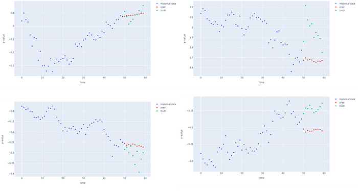
The forecasts for first node (Google) at 4 different points from the test dataset is actually better than I thought. My humble opinion on the stock market price prediction is that the stocks are determined by the events of the real world and this is not captured in the historical values. Future stock prices cannot be predicted by purely autoregression of historical values. But I have no experience with financial forecasting so will leave it there. That brings us to the end of discussion about the ST-GNNs, thank you for taking the time to read, I hope you found it insightful!

Unless otherwise noted, all images are by the author

Join thousands of data leaders on the AI newsletter. Join over 80,000 subscribers and keep up to date with the latest developments in AI. From research to projects and ideas. If you are building an AI startup, an AI-related product, or a service, we invite you to consider becoming a sponsor.

Published via Towards AI