Forecasting Time Series Data: Netflix Stock Price Prediction

Author(s): Alison Yuhan Yao

Originally published on Towards AI.

ARIMA-(G)ARCH models with MiniTab and R

The Netflix stock price has been quite volatile recently, which makes the prediction of the time series data very interesting. In this blog, I will use ARIMA-(G)ARCH models for prediction, Minitab for plotting, and R for model selection. (Because of the instructions of this class project, I will have to comply with some restrictions.)

Some prior knowledge before reading this blog includes:

• ARIMA model
• ARCH and GARCH models

Data Description

This project uses the daily stock price of Netflix from 2002–05–23 to 2022–03–18 (4991 observations) for the time series forecast. The 2022–03–18 data is the latest entry from Yahoo Finance as of the time I obtained the dataset. The head of the table is shown below:

I will leave out the last data point, which is the data for 2022–03–18 for the ARIMA-(G)ARCH modeling. Therefore, n=4991–1=4990 and I will be using the Adj Close data from 2002–05–23 to 2022–03–17.

ARIMA modeling

The time series plots of Netflix stock price (Adj Close), DifNetflix, LogNetflix, and DifLogNetflix are as follows:

There is strong evidence that Netflix has level-dependent volatility. Netflix stock prices are more volatile in recent years. Taking log can help us mitigate level-dependent volatility and linearize the plot, as the volatility of DifLogNetflix does not seem to depend on a level anymore.

For choosing an ARIMA(p,d,q) model, we need to first determine the value of d and see how many times we need to difference the data to make it stationary. The ACF and PACF plot of LogNetflix is as follows:

The ACF plot of LogNetflix indicates a hanging behavior and the PACF plot of LogNetflix cuts off after lag 1, so LogNetflix is non-stationary. We need to difference the data.

The ACF and PACF plots of DifLogNetflix show that differencing once seems to make the data stationary, as there are no statistically significant lags.

To double-check if d=1, we can difference the data again and look for a sign of over-differencing.

Indeed, differencing twice shows strong evidence of over-differencing as the PCF of Dif2LogNetflix is statistically significantly negative at lag 1 and close to -0.5. Therefore, we conclude that d=1 in the ARIMA model. The ACF plot of DifLogNetflix suggests an ARIMA(0,1,4) model, while the PACF of DifLogNetflix suggests an ARIMA(4,1,0) model.

Now, we need to select the p and q in the ARIMA model. Let’s pick p,q = 0,1,2 arbitrarily (because of the principle of parsimony) and compare AICc. The formula for AICc is as follows:

The SS means the sum of squared error and it can be obtained from Minitab output. We know N = n–d = 4990–1 = 4989.

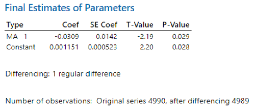
ARIMA(0,1,1) with constant gives us the smallest AICc value, so we choose ARIMA(0,1,1) with constant. The Minitab output for ARIMA(0,1,1) with constant is:

Both the MA1 coefficient and the constant are statistically significant, with p-values less than 0.05. Therefore, if we denote {x_t} as the time series of Netflix, {y_t} as LogNetflix and {z_t} as DifLogNetflix. The best estimate of the MA1 coefficient is -0.0309 and that of the constant is 0.001151. Therefore, the fitted model is

where z_t = y_t-y_{t-1} = log(x_t)-log(x_{t-1}).

The one step ahead forecast and 95% forecast interval are as follows:

The time series plot of the residuals is:

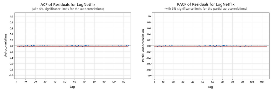
The residuals look relatively random, with only a few with absolute values over 0.3. The ACF and PACF plots of the residuals are as follows:

There aren’t many statistically significant lags in the residuals, meaning that the residuals look uncorrelated. The ACF and PACF of squared residuals are:

However, the squared residuals have multiple lags that are statistically significant, meaning that the residuals are not independent. Also, we can see from the time series plot of the residuals that the variance is not constant. There exists evidence of conditional heteroscedasticity.

Before doing the (G)ARCH modeling, we need to save the residual information from Minitab to a txt file and import it into R.

# read file & check head
res = scan("RES.txt", what="list")
head(res)# clean up data & convert data type
res = res[-c(1,2)]
res = as.numeric(res)
head(res)

(G)ARCH modeling

ARCH(q)

To select the ARCH(q) model with q ranging from 0 to 10, we can calculate the AICc. The formula for AICc changes here:

The values of logLik can be obtained from R.

library(tseries)# check different ARCH models
for (i in 1:10){
 print(paste0('model ARCH(', i, ')'))
 model = garch(res, c(0,i), trace=F)
 print(summary(model))
 print(logLik(model))
}# ARCH(0) model has to be manually calculated
# model = garch(res, c(0,0), trace=F) is going to give an error
N = 4989
print(paste0('log Lik.', -0.5*N*(1+log(2*pi*mean(res^2)))))

Again, we know N = n–d = 4990–1 = 4989, so we have:

GARCH(1,1)

We can also consider the GARCH(1,1) model due to the principle of parsimony. We have logLik = 9799.593 (q=2) and the corresponding AICc is -19593.18118555667. GARCH(1,1) yields the smallest AICc, so we choose GARCH(1,1).

# compared with GARCH(1,1) model
model=garch(res,c(1,1), trace=F)
print(summary(model))
print(logLik(model))

The p-values are not correct because they are for a 2-tailed test. We should look at half of the presented p-values, but they are so small that half of any of these p-values is strongly statistically significant. Therefore, a0, a1, and b1 are all statistically significant. However, the Jarque Bera test has a p-value less than 0.05, which indicates that the conditional distribution of GARCH residuals is not normally distributed. The Ljung-Box test has a p-value greater than 0.05, which means that the GARCH residuals are not correlated. But overall, the model is inadequate.

To write the complete form of the chosen GARCH(1,1) model, we have ω=0.000005875, α=0.01425, and β=0.9814. Therefore, the complete form is

The unconditional variance is

We know from the residual data that ϵ_4990=0.035765. We also know that h_4990=0.00138539642318183. Therefore,
h_4991=0.000005875 + 0.01425 × 0.035765² + 0.9814 × 0.00138539642318183 = 0.001383731.

From the ARIMA(0,1,1) model, we know that f_4990,1=5.91954. The 95% forecast interval of the ARIMA-GARCH model is, therefore:

Compared to the ARIMA(0,1,1) model, which has a 95% forecast interval of (5.84927, 5.98981), the ARIMA-GARCH model has a wider forecast interval.

The 5th percentile of the conditional distribution of the next period’s log exchange rate is:

Now we calculate the conditional variance ht:

# calculate ht
ht = model$fit[,1]^2
ht[1:5] # has NA
write(c('ht', '*', ht), '../htfile.txt', 1)

The time series plot of ht is:

The ht from 2002/5/23 to 2014/4/14 is more volatile than later ht. Bursts of high volatility reside between 2002/5/23 to 2014/4/14, with the highest volatility residing between 2022/5/23 to 2005/5/9.

Compared with the time series plot of LogNetflix, it seems that these bursts of high volatility do agree with those found from the examination of the time series plot of the log exchange rates themselves.

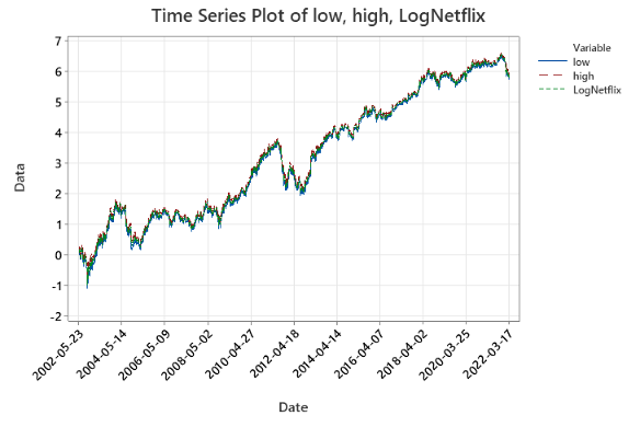
The time series plot of logNetflix and one-step ahead 95% forecast intervals is as follows:

According to the plot, LogNetflix is mostly between low and high, so the forecast interval is quite accurate. However, since the ARIMA-GARCH parameters are estimated from the entire data set, not just the observations up to the time at which the forecast is to be constructed, the performance may be somewhat better here than in an actual forecasting context, so the practical usefulness is somewhat questionable for x_1 to x_4990. However, x_4991 was not utilized in building the ARIMA-GARCH model, so the forecast for x_4991 is more practically useful.

The test tells us that the p-value is smaller than 0.005, so archres are not normally distributed. The s-shaped plot is an indicator that a heavier tail, which means that the model does not seem to have adequately described the leptokurtosis in the data.

There are 209 failures in prediction intervals, which is about 209/4988 = 4.19% of all intervals.

Performance Check

For LogNetflix, the 95% forecast interval of the ARIMA model is (5.84927, 5.98981), which corresponds to an interval of (347.89, 399.339) for Netflix. x_4991=380.6 is within the forecast interval.

The 95% forecast interval of the ARIMA-GARCH model is (5.846631, 5.992449), which corresponds to an interval of (346.0665, 400.39398) for Netflix. x_4991=380.6 is within the forecast interval.

The ARIMA interval and ARIMA-GARCH interval are very similar. Both forecast intervals seem neither too wide nor too narrow. The ARIMA-GARCH interval is slightly wider to adapt to the recent higher volatility because ARIMA-GARCH is adaptive, but ARIMA is not.

Join thousands of data leaders on the AI newsletter. Join over 80,000 subscribers and keep up to date with the latest developments in AI. From research to projects and ideas. If you are building an AI startup, an AI-related product, or a service, we invite you to consider becoming a sponsor.

Published via Towards AI