Fishing: The Bayesian Way of Analyzing Zero-inflated Data

Author(s): Dr. Marc Jacobs

Originally published on Towards AI the World’s Leading AI and Technology News and Media Company. If you are building an AI-related product or service, we invite you to consider becoming an AI sponsor. At Towards AI, we help scale AI and technology startups. Let us help you unleash your technology to the masses.

In past posts, I have shown several ways to apply Bayesian analysis for mostly normally distributed data. In this example, I want to use a discrete response, and what better distribution to start with than an inflated one. You read correctly — this post will be about modeling, in a Bayesian way, a zero-inflated response.

A zero-inflated response distribution is one in which there are more zero’s than you would normally like, but they are there. Hence, you need to deal with them and there are various ways to cope. The most straightforward is the application of a zero-inflated model or applying a hurdle model. They work a bit differently, but what they do have in common is that you split your modeling into a part where you model the zero’s, and a part in which you model the rest. This will be done via two separate models (the hurdle) or via a mixture distribution (the zero-inflated model).

Once again, the codes are at the bottom to not contaminate the story. Also, the codes, in the end, show more information than what I have here. The trick is to run everything I did and augment it. Not just follow my steps.

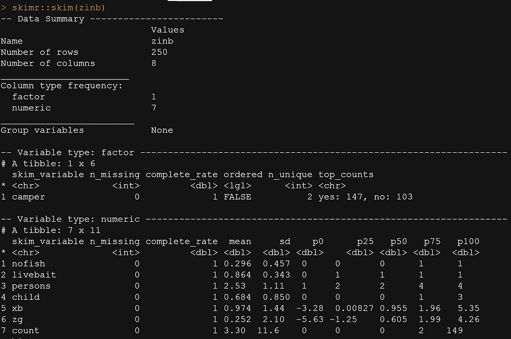
Alright, so let's go and take a look at the dataset, which can be found here. As you can see, we have a lot of discrete data, both binary as well as ordinal or multinomial. Discrete data is fun to analyze albeit a bit challenging, but should not be a big issue for any analyst. Just think proportions | probabilities | and rates and you will be fine.

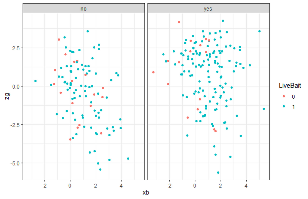
Next up is the drawing part in which I want to see what I have. The dataset has information on fish, of course, and the metric that matters the most is the count. We are working with count data here.

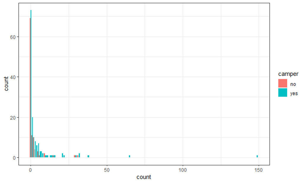
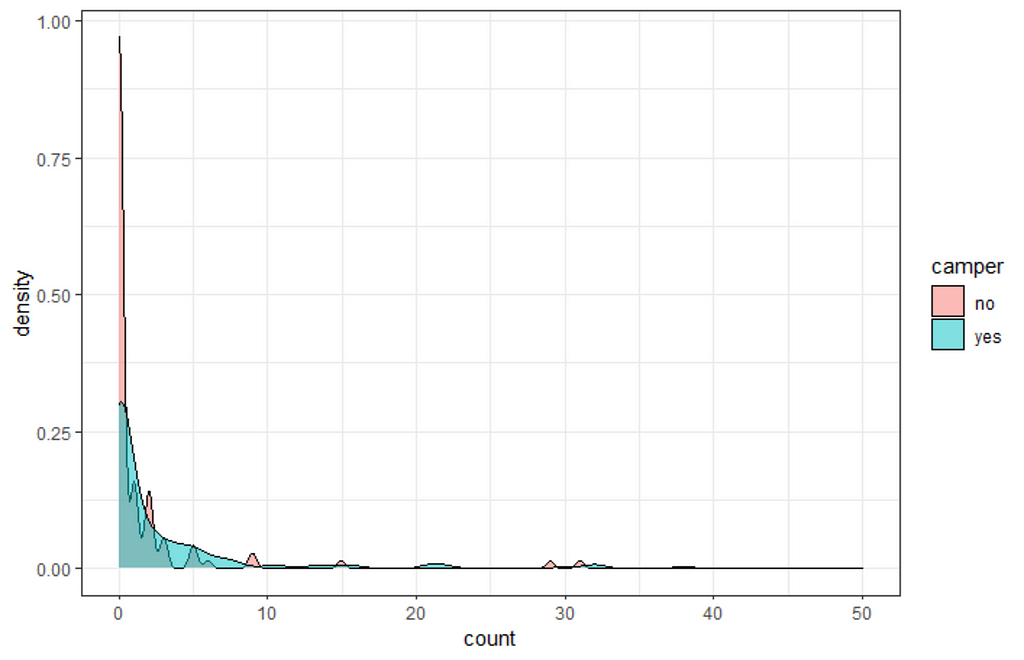
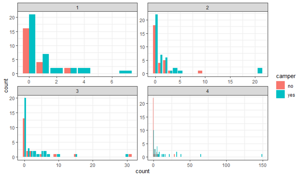
The zero-inflated nature of the data becomes immediately apparent (although you could already see it coming in the dotplot) when doing a distribution plot. The spike at the beginning will give you problems if you try and analyze via the standard Poisson, or even when using a Gamma-Poisson (Negative Binomial).

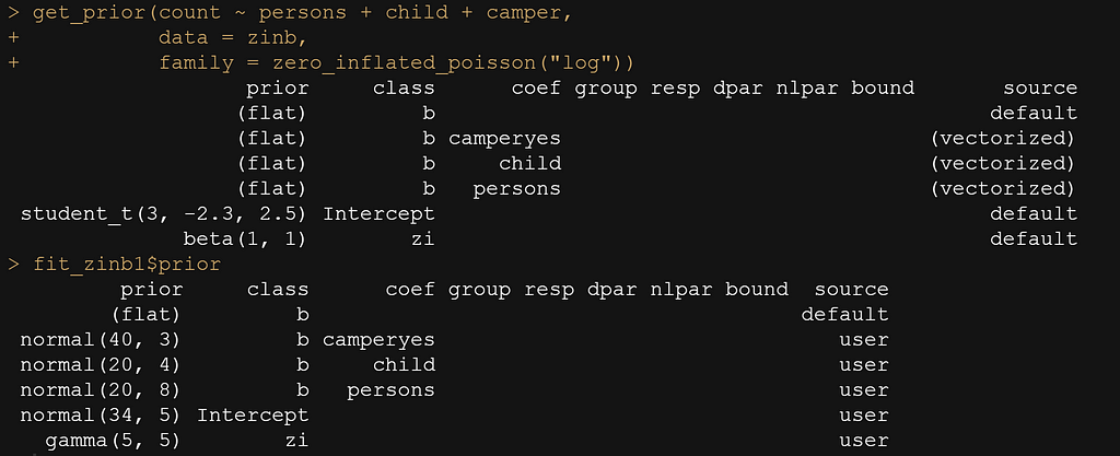
Of to the modeling part. Of course, I am going Bayesian which means I will have to deal with the three musketeers of Bayesian analysis: prior, likelihood, and posterior. Since I know that the response resembles a zero-inflated distribution, I can ask the brms package to show me the priors the model would automatically assume. Thereby seeing how it wants me to feed the hyperparameters should I decide to bring my own priors (of course I will!).

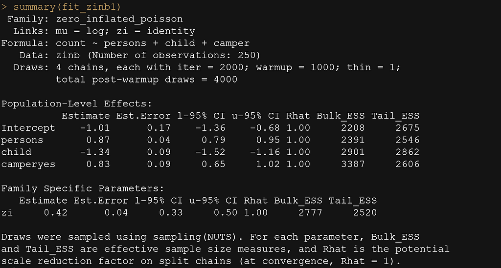
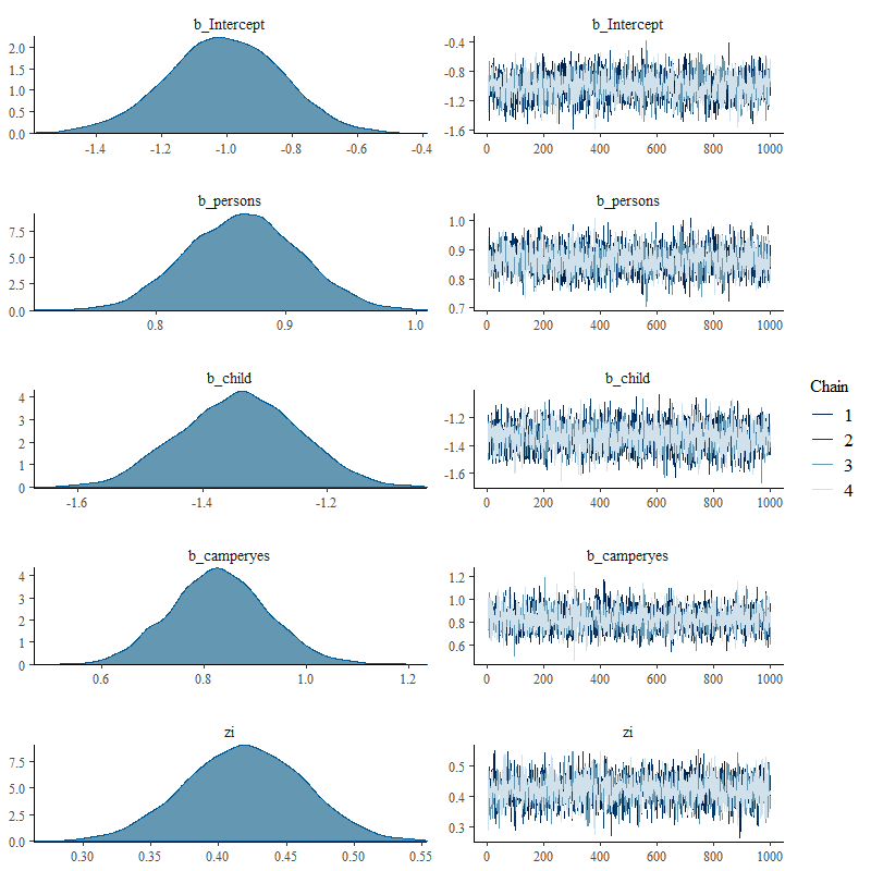
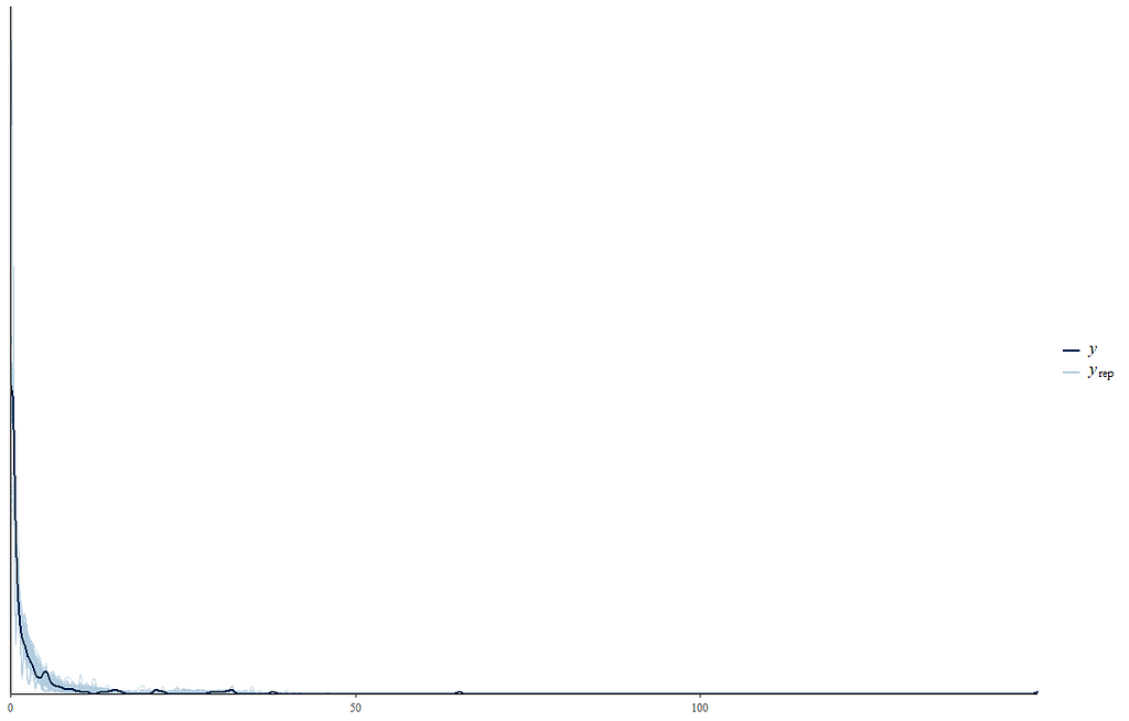
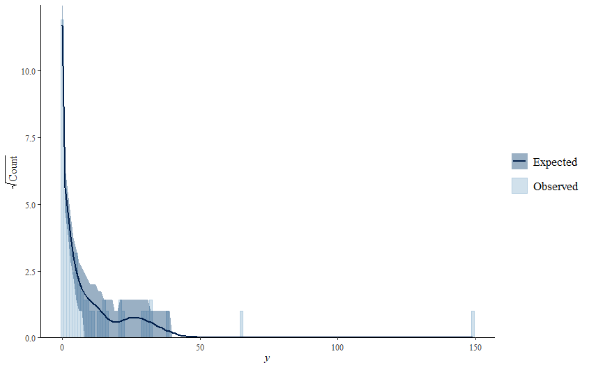
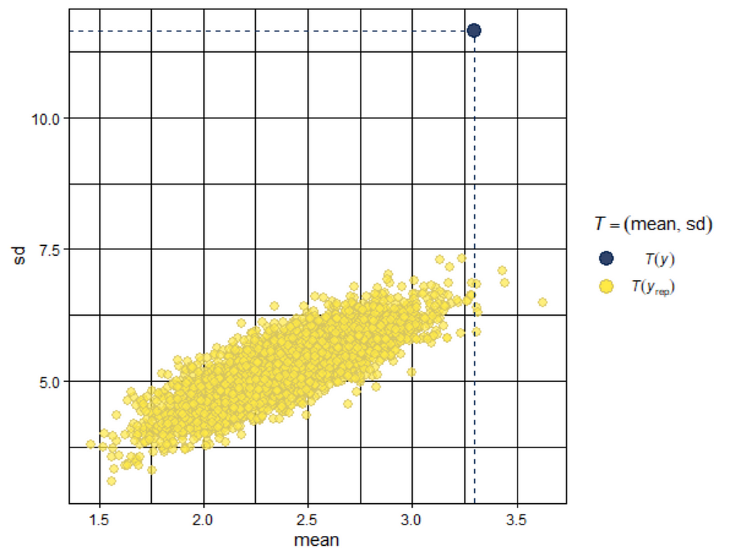
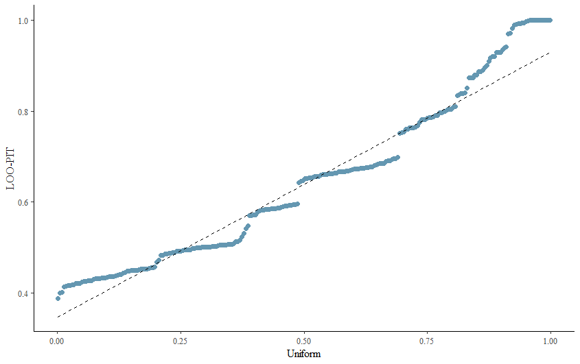
When it comes to Bayesian Analysis you do want to see that your model is able to approximate the underlying distribution via which the data came to exist (that sounds a bit paradoxical — distribution is a man-made construct). Hence, what you want to see when checking the appropriateness of the Bayesian model is that the chains converged nicely and that the distribution in the model used was appropriately sufficient. We can do that by looking at the PIT which transforms the data into a uniform distribution. If the QQ-plot shows that the samples are on the diagonal line, the underlying distribution (which is not uniform here) is probably what thought it would be, which is a zero-inflated distribution. The lines are not perfect here, but I will give it a pass. Not the easiest data to the model.

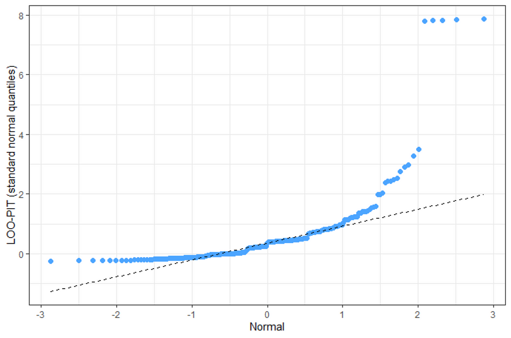
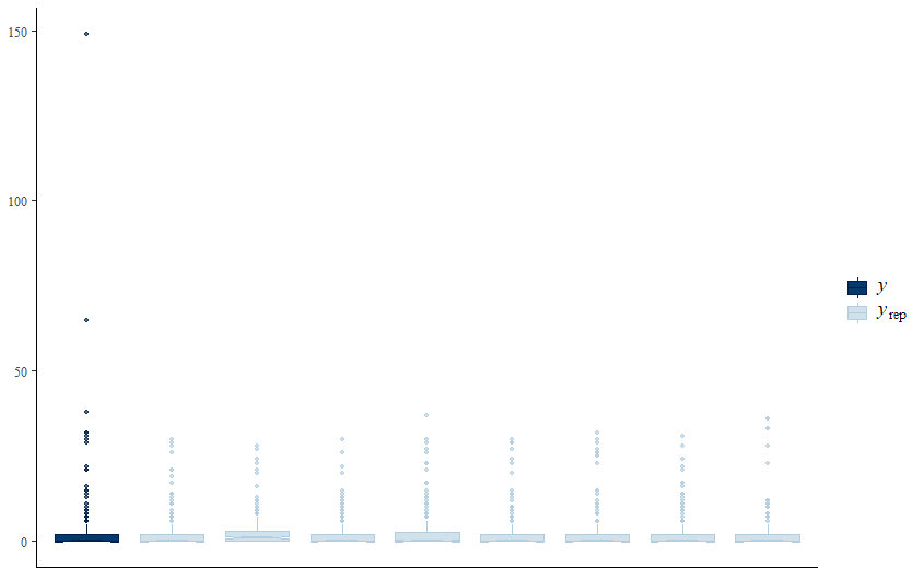
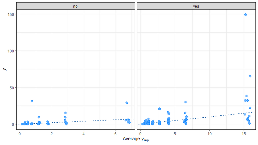
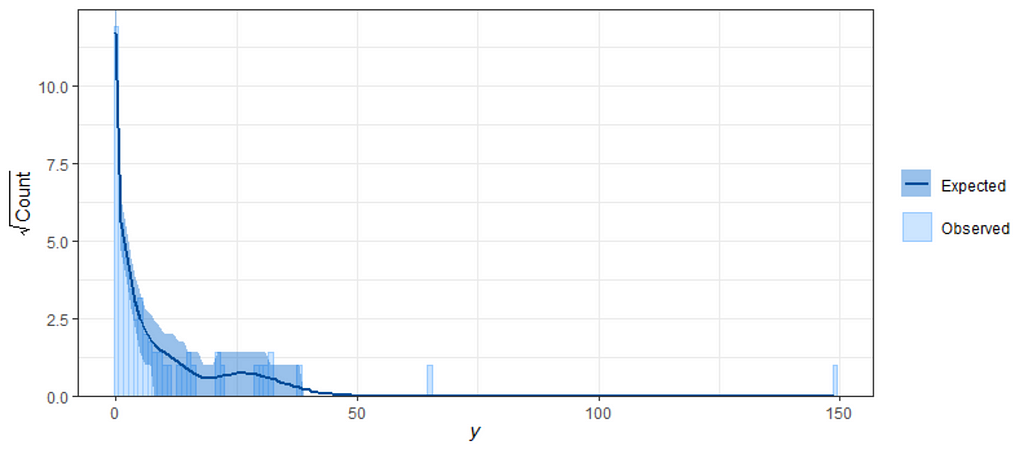
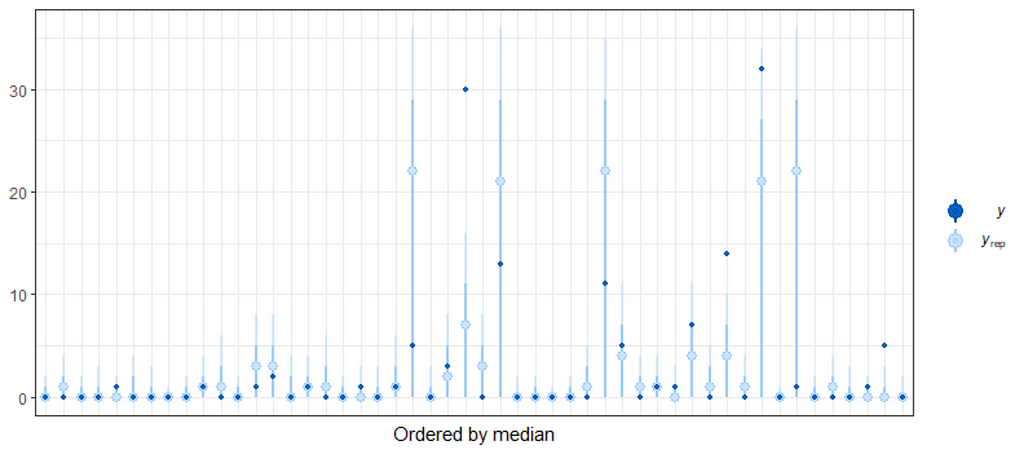
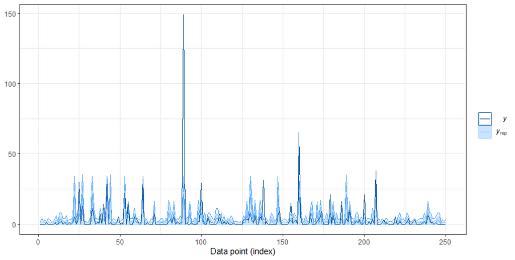
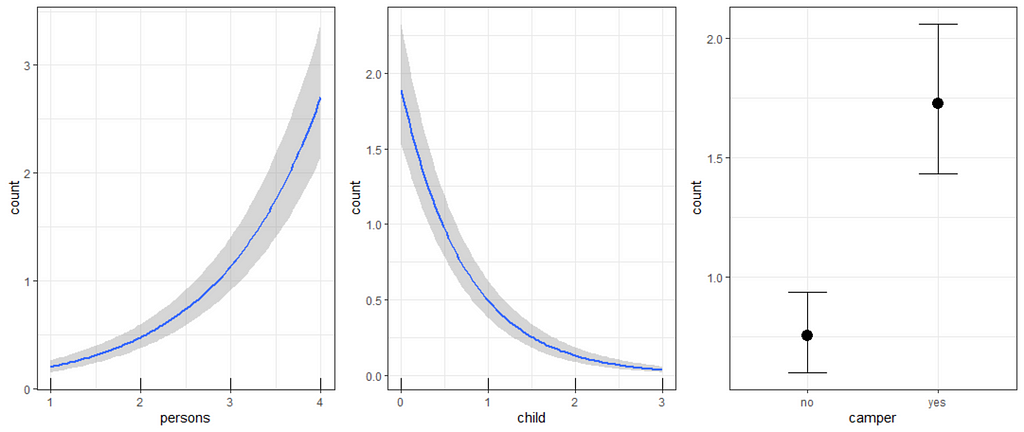
So, from the above, it seems the model is quite able to model the data, and hence we can use the model to take a better look at the underlying relationships which you find by extracting a conditional distributions plot. What you see below is the relationship between the variables persons, child, and camper with the count.

I hope this example was sufficient to get you underway with modeling a Zero-Inflated dataset. Go through the codes down below and please let me know if something is amiss!

Enjoy!

Fishing: The Bayesian Way of Analyzing Zero-inflated Data was originally published in Towards AI on Medium, where people are continuing the conversation by highlighting and responding to this story.

Join thousands of data leaders on the AI newsletter. It’s free, we don’t spam, and we never share your email address. Keep up to date with the latest work in AI. From research to projects and ideas. If you are building an AI startup, an AI-related product, or a service, we invite you to consider becoming a sponsor.

Published via Towards AI