Complete Guide to Pandas DataFrame with real-time use case

Author(s): Muttineni Sai Rohith

Originally published on Towards AI the World’s Leading AI and Technology News and Media Company. If you are building an AI-related product or service, we invite you to consider becoming an AI sponsor. At Towards AI, we help scale AI and technology startups. Let us help you unleash your technology to the masses.

Complete Guide to Pandas Dataframe With Real-time Use Case

After my Pyspark Series — where readers are mostly interested in Pyspark Dataframe and Pyspark RDD, I got suggestions and requests to write on Pandas DataFrame, So that one can compare between Pyspark and Pandas not in consumption terms but in Syntax terms. So today in this article, we are going to concentrate on functionalities of Pandas DataFrame using Titanic Dataset.

Pandas refer to Panel Data/ Python Data analysis. In general terms, Pandas is a python library used to work with datasets.

DataFrame in pandas is a two-dimensional data structure or a table with rows and columns. DataFrames provides functions for creating, analyzing, cleaning, exploring, and manipulating data.

Installation:

pip install pandas

Importing pandas:

import pandas as pd
print(pd.__version__)

This will print the Pandas version if the Pandas installation is successful.

Creating DataFrame:

Creating an empty DataFrame —

df=pd.DataFrame()
df.head(5) # prints first 5 rows in DataFrame

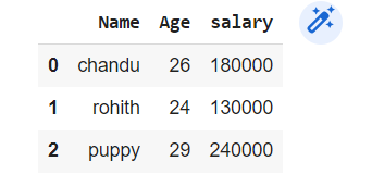
Creating DataFrame from dict—

employees = {'Name':['chandu','rohith','puppy'],'Age':[26,24,29],'salary':[180000,130000,240000]}

df = pd.DataFrame(employees)
df.head()

Creating Dataframe from a list of lists —

employees = [['chandu',26,180000], ['rohith', 24, 130000],['puppy', 29 ,240000]]

df = pd.DataFrame(employees, columns=["Name","Age","Salary"])
df.head()

Importing data from CSV File mentioned here.

df = pd.read_csv("/content/titanic_train.csv")

df.head(5)

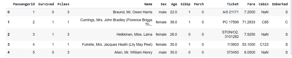
As shown above, df.head(n) will return the first n rows from DataFrame while df.tail(n) will return the last n rows from DataFrame.

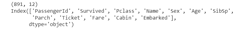
print(df.shape)  #prints the shape of DataFrame - rows * columns

print(df.columns)  #returns the column names

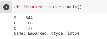
value_counts()— returns the unique values with their counts in a particular column.

df["Embarked"].value_counts()

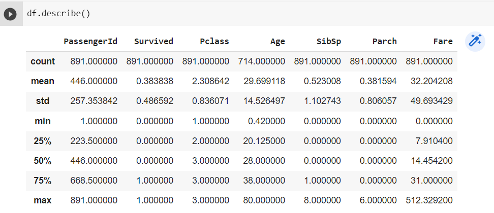
df.describe() — Getting information about all numerical columns in DataFrame

df.describe()

df.info() — returns the count and data type of all columns in DataFrame

df.info()

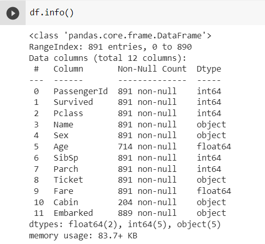
As seen above, There is the count of Age and Cabin is less than 891, so there might be missing values in those columns. We can also see the dtype of the columns in the DataFrame.

Handling Missing Values

Getting the count of missing Values —

df.isnull().sum()

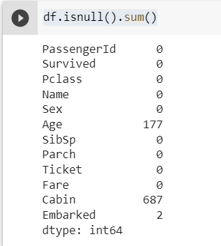
As seen above, columns “Age”, “Cabin” and “Embarked” has missing values.

To get the percentage of missing values —

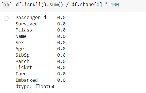
df.isnull().sum() / df.shape[0] * 100

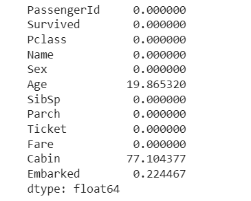
As we can see, the missing values percentage of Cabin is more than 75%, so let’s drop the column.

df=df.drop(['Cabin'],axis=1)

The above command is used to drop certain columns from DataFrame.

Imputing Missing Values

Let’s impute the missing values in the Age column by mean Value.

df['Age'].fillna(df['Age'].mean(),inplace=True)

And impute the missing values in an Embarked column by Mode Value.

df['Embarked'].fillna(df['Embarked'].mode().item(),inplace=True)

In the above example, .item() is used as we are dealing with a string column. I think all the missing Values are handled, let’s check —

Renaming Columns

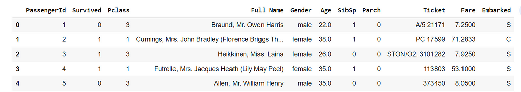
df=df.rename(columns={'Sex':'Gender','Name':'Full Name'})
df.head()

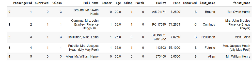
Adding/Modifying Columns

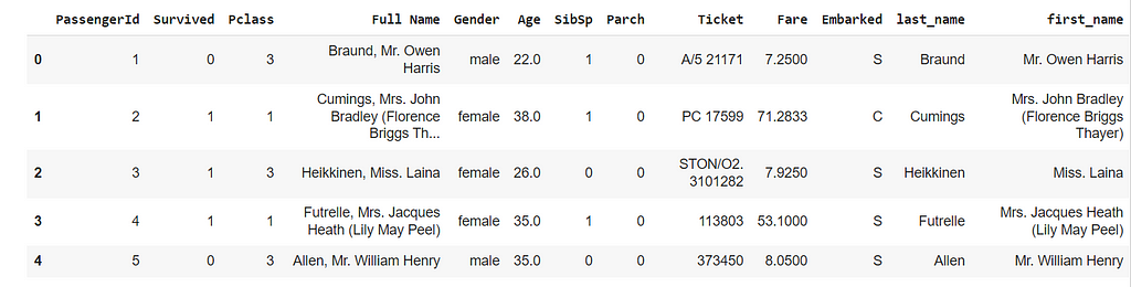
df['last_name']=df['Full Name'].apply(lambda x: x.split(',')[0])

df['first_name']=df['Full Name'].apply(lambda x: ' '.join(x.split(',')[1:]))

df.head(5)

Adding Rows — we use df.append() method to add the rows

row=dict({'Age':24,'Full Name':'Rohith','Survived':'Y'})

df=df.append(row,ignore_index=True)

df.tail()

A new row is created, and NaN values are initialized for columns with No Values

using loc() method:

df.loc[len(df.index)]=row
df.tail()

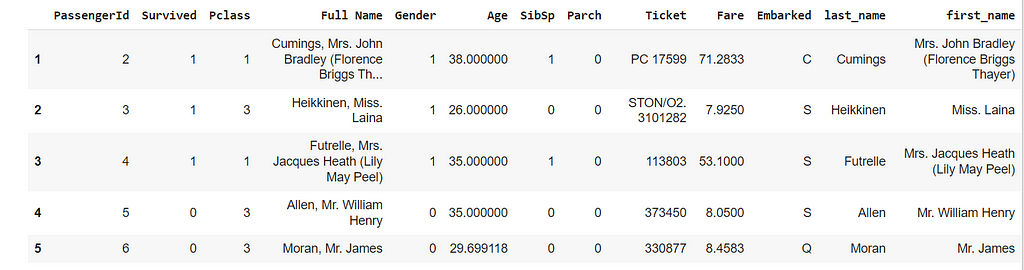
Deleting Rows

using df.index() method —

df=df.drop(df.index[-1],axis=0) # Deletes last row
df.head()

Encoding Columns

For most of the machine learning algorithms, we should have numerical data instead of Data in String format. So Encoding data is a must operation.

df['Gender']=df['Gender'].map({"male":'0',"female":"1"})

df.head(5)

As this process becomes hectic for all columns if we use the above method, there are many methods such as LabelEncoder, OneHotEncoder, and MultiColumnLabelEncoder available to Encode the DataFrames. They are explained clearly in the below Article —

Encoding Methods to encode Categorical data in Machine Learning

Filtering the Data

Selecting the data only when age is greater than 25.

df[df["Age"]> 25].head(5)

Similarly we can use > , < and == operations.

df[(df["Age"]< 25) & (df["Gender"]=="1")].head(5)

selecting data when Age is less than 25 and Gender is 1. In the above way, we can also filter multiple columns.

apply() function:

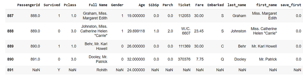
Let’s assume that people aged less than 15 and greater than 60 are going to be saved first. Let’s make a save_first column using apply() function.

def save_first(age):
    if age<15:
        return 1
    elif age>=15 and age<60:
        return 0
    elif age>=60:
        return 1

df['save_first']=df['Age'].apply(lambda x: save_first(x))

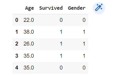
Selecting particular Columns and Rows:

df_1 = df[['Age','Survived','Gender']]

df_1.head()

using .iloc() — It uses numerical indexes to return particular rows and columns in the DataFrame

df_2 = df.iloc[0:100,:]

df_2.head()

returns the first 100 rows and all columns in DataFrame

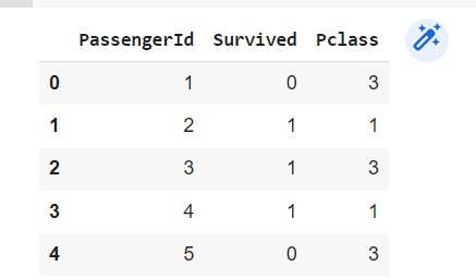
df_2 = df.iloc[0:100, [0,1,2]]

df_2.head()

returns first 100 rows and first 3 columns in DataFrame

.loc() function — similar to .iloc() but it uses Column Names instead of numerical indexes.

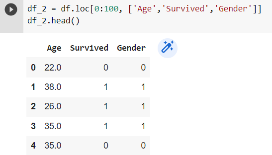
df_2 = df.loc[0:100, ['Age','Survived','Gender']]

df_2.head()

Sorting

We can perform sorting operations in DataFrame using sort_values() method.

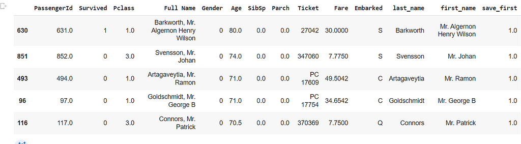
df=df.sort_values(by=['Age'],ascending=False)

df.head()

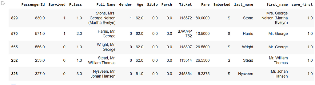
We can also use multiple columns — first sorts by the first column, followed by the second column.

df=df.sort_values(by=['Age', 'Survived'],ascending=False)

df[15:20]

Join

Join is nothing but combining multiple DataFrames based on a particular column.

Let's perform 5 types of Joins — cross, inner, left, right, and outer

cross join — also known as a cartesian join, which returns all combinations of rows from each table.

cross_join = pd.merge( df1 , df2 ,how='cross')

inner join — returns only those rows that have matching values in both Dataframes.

inner_join = pd.merge( df1 , df2 ,how='inner', on='column_name')

left join — returns all the rows from the first DataFrame, if there are no matching values, then it returns null Values for Second DataFrame

left_join = pd.merge( df1 , df2 ,how='left', on='column_name')

right join — returns all the rows from the Second DataFrame. If there are no matching values, then it returns null Values for first DataFrame

right_join = pd.merge( df1 , df2 ,how='right', on='column_name')

outer join — returns all the rows from both first and Second DataFrames. In case there is no match in the first Dataframe, Values in the Second DataFrame will be null and ViceVersa

outer_join = pd.merge( df1 , df2 ,how='outer', on='column_name')

GroupBy()

This method is used to group a dataframe based on a few columns.

groups = df.groupby(['Survived'])

groups.get_group(1)

get_group() method is used to get the data belonging to a certain group.

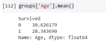
GroupBy() generally used with mathematical functions such as mean(), min(), max() etc.,

groups['Age'].mean()

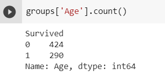
groups['Age'].count()

groups['Age'].min()
groups['Age'].max()

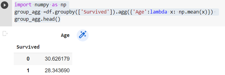
Using .agg() function

import numpy as np

group_agg =df.groupby(['Survived']).agg({'Age':lambda x: np.mean(x)})

group_agg.head()

So I think I have covered most of the basic concepts related to Pandas DataFrame.

Happy Coding…

---

Complete Guide to Pandas DataFrame with real-time use case was originally published in Towards AI on Medium, where people are continuing the conversation by highlighting and responding to this story.

Join thousands of data leaders on the AI newsletter. It’s free, we don’t spam, and we never share your email address. Keep up to date with the latest work in AI. From research to projects and ideas. If you are building an AI startup, an AI-related product, or a service, we invite you to consider becoming a sponsor.

Published via Towards AI