Analyzing Ordinal Data in SAS — Poisson and Negative Binomial distribution

Author(s): Dr. Marc Jacobs

Originally published on Towards AI.

Analyzing Ordinal Data in SAS — Poisson and Negative Binomial distribution

This post is an extension to an introductory post on using PROC GLIMMIX in SAS. I already showed how to analyze ordinal data using the multinomial distribution, and the binary, binomial, and beta distribution. In this post, I will use the Poisson Distribution of which I have posted earlier as well. This post will extend those posts by analyzing the same dataset — diarrhea scores measured in pigs across time. Here, diarrhea is measured subjectively using an ordinal scoring system.

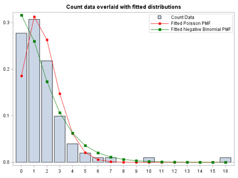
So, this post will be rather short and must be seen more as an extension to earlier PROC GLIMMIX posts. Below you will see a plot of count data overlaid with fitted distributions. Two of the most well-known and often used distribution are the Poisson and the Negative-Binomial of which the latter is more flexible. This is because the Negative-Binomial model is a mixture of two distributions — the Poisson and the Gamma distribution.

As you can see in the plot below, the negative binomial can fit the data better, yet will overestimate the number of zero’s. When dealing with counts, those zero’s can be troublesome which has led to the application of Zero-Inflated models, which I will not discuss here.

By definition count data are a rate which normally follows a Poisson distribution. Here, in this example, we counted the amount of diarrhea across the total time period. This means that, for an ordinal scale, we need to dichotomize it. Otherwise we do not have the ‘events’ necessary to model the rate.

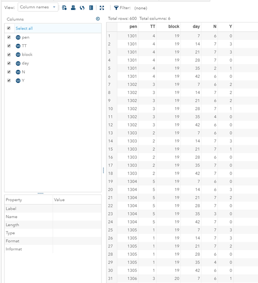
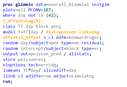
Using the Binomial Distribution, you need to specify a nominator (Y) and a denominator (N). Using the Poisson distribution, you need to specify a nominator (Y) and an offset variable (N). The offset needs to be on the log scale. This offset is very important — it gives the rate the other metric it needs to be a rate.

This can be seen by using the table below. The choice to include no feces as no diarrhea or no missing has an effect on the rate, since the offset changes. This is normal since the denominator changes as well.

In the introductory post, I already mentioned the danger of overdispersion which is common when using the Poisson distribution. This is because the Poisson is a single parameter distribution — the mean equals the variance.

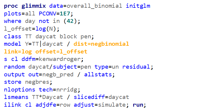
Now, lets see how a negative binomial looks at the data. Since the Poisson analysis already showed an absence of overdispersion, I know for sure that the Negative Binomial will detect the same. Hence, we can go straight to the analysis itself.

Lets use a different dataset in which we know the data is more placed apart.

In summary, the Poisson distribution models count data. To analyze diarrhea using the Poisson distribution, you can use the dataset in the format used for the Binomial Distribution. Since the Poisson models a rate, you need to include an offset variable, which is the denominator in the equation. Using the Poisson, you always need to watch out for overdispersion. A good replacement for the Poisson distribution is the Negative Binomial distribution

Join thousands of data leaders on the AI newsletter. Join over 80,000 subscribers and keep up to date with the latest developments in AI. From research to projects and ideas. If you are building an AI startup, an AI-related product, or a service, we invite you to consider becoming a sponsor.

Published via Towards AI