Monte Carlo Simulation An In-depth Tutorial with Python

An in-depth tutorial on the Monte Carlo Simulation methods and applications with Python

Author(s): Pratik Shukla, Roberto Iriondo

What is the Monte Carlo Simulation?

A Monte Carlo method is a technique that uses random numbers and probability to solve complex problems. The Monte Carlo simulation, or probability simulation, is a technique used to understand the impact of risk and uncertainty in financial sectors, project management, costs, and other forecasting machine learning models.

Risk analysis is part of almost every decision we make, as we constantly face uncertainty, ambiguity, and variability in our lives. Moreover, even though we have unprecedented access to information, we cannot accurately predict the future.

The Monte Carlo simulation allows us to see all the possible outcomes of our decisions and assess risk impact, in consequence allowing better decision making under uncertainty.

In this article, we will go through five different examples to understand the Monte Carlo Simulation methods.

📚 Resources: Google Colab Implementation | GitHub Repository 📚

Applications:

• Finance.
• Project Management.
• Energy.
• Manufacturing.
• Engineering.
• Research and Development.
• Insurance.
• Oil and Gas.
• Transportation.
• Environment.
• And others.

Examples:

1. Coin Flip Example.
2. Estimating PI Using Circle and Square.
3. Monty Hall Problem.
4. Buffon’s Needle Problem.
5. Why Does the House Always Win?

a. Coin Flip Example:

While flipping a coin:

Next, we are going to prove this formula experimentally using the Monte Carlo Method.

Python Implementation:

1. Import required libraries:

2. Coin flip function:

3. Checking the output of the function:

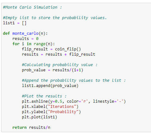
4. Main function:

5. Calling the main function:

As shown in figure 8, we show that after 5000 iterations, the probability of getting a tail is 0.502. Consequently, this is how we can use the Monte Carlo Simulation to find probabilities experimentally.

b. Estimating PI using circle and square :

To estimate the value of PI, we need the area of the square and the area of the circle. To find these areas, we will randomly place dots on the surface and count the dots that fall inside the circle and dots that fall inside the square. Such will give us an estimated amount of their areas. Therefore instead of using the actual areas, we will use the count of dots to use as areas.

In the following code, we used the turtle module of Python to see the random placement of dots.

Python Implementation:

1. Import required libraries:

2. To visualize the dots:

3. Initialize some required data:

4. Main function:

5. Plot the data:

6. Output:

As shown in figure 17, we can see that after 5000 iterations, we can get the approximate value of PI. Also, notice that the error in estimation also decreased exponentially as the number of iterations increased.

📚 Check out an overview of machine learning algorithms for beginners with code examples in Python. 📚

3. Monty Hall Problem:

Suppose you are on a game show, and you have the choice of picking one of three doors: Behind one door is a car; behind the other doors, goats. You pick a door, let’s say door 1, and the host, who knows what’s behind the doors, opens another door, say door 3, which has a goat. The host then asks you: do you want to stick with your choice or choose another door? [1]

Is it to your advantage to switch your choice of door?

Based on probability, it turns out it is to our advantage to switch the doors. Let’s find out how:

Initially, for all three gates, the probability (P) of getting the car is the same (P = 1/3).

Now assume that the contestant chooses door 1. Next, the host opens the third door, which has a goat. Next, the host asks the contestant if he/she wants to switch the doors?

We will see why it is more advantageous to switch the door:

In figure 19, we can see that after the host opens door 3, the probability of the last two doors of having a car increases to 2/3. Now we know that the third door has a goat, the probability of the second door having a car increases to 2/3. Hence, it is more advantageous to switch the doors.

Now we are going to use the Monte Carlo Method to perform this test case many times and find out its probabilities in an experimental way.

Python Implementation:

1. Import required libraries:

2. Initialize some data:

3. Main function:

4. Calling the main function:

5. Output:

In figure 24, we show that after 1000 iterations, the winning probability if we switch the door is 0.669. Therefore, we are confident that it works to our advantage to switch the door in this example.

4. Buffon’s Needle Problem:

A French nobleman Georges-Louis Leclerc, Comte de Buffon, posted the following problem in 1777 [2] [3].

Suppose that we drop a short needle on a ruled paper — what would be the probability that the needle comes to lie in a position where it crosses one of the lines?

The probability depends on the distance (d) between the lines of the ruled paper, and it depends on the length (l) of the needle that we drop — or rather, it depends on the ratio l/d. For this example, we can interpret the needle as l ≤ d. In short, our purpose is that the needle cannot cross two different lines at the same time. Surprisingly, the answer to the Buffon’s needle problem involves PI.

Here we are going to use the solution of Buffon’s needle problem to estimate the value of PI experimentally using the Monte Carlo Method. However, before going into that, we are going to show how the solution derives, making it more interesting.

Theorem:

If a short needle, of length l, is dropped on a paper that is ruled with equally spaced lines of distance d ≥ l, then the probability that the needle comes to lie in a position where it crosses one of the lines is:

Proof:

Next, we need to count the number of needles that crosses any of the vertical lines. For a needle to intersect with one of the lines, for a specific value of theta, the following are the maximum and minimum possible values for which a needle can intersect with a vertical line.

1. Maximum Possible Value:

2. Minimum Possible Value:

Therefore, for a specific value of theta, the probability for a needle to lie on a vertical line is:

The above probability formula is only limited to one value of theta; in our experiment, the value of theta ranges from 0 to pi/2. Next, we are going to find the actual probability by integrating it concerning all the values of theta.

Estimating PI using Buffon’s needle problem:

Next, we are going to use the above formula to find out the value of PI experimentally.

Now, notice that we have the values for l and d. Our goal is to find the value of P first so that we can get the value of PI. To find the probability P, we must need the count of hit needles and total needles. Since we already have the count of total needles, the only thing we require now is the count of hit needles.

Below is the visual representation of how we are going to calculate the count of hit needles.

Python Implementation:

1. Import required libraries:

2. Main function:

3. Calling the main function:

4. Output:

As shown in figure 37, after 100 iterations we are able to get a very close value of PI using the Monte Carlo Method.

5. Why Does the House Always Win?

How do casinos earn money? The trick is straightforward — “The more you play, the more they earn.” Let us take a look at how this works with a simple Monte Carlo Simulation example.

Consider an imaginary game in which a player has to choose a chip from a bag of chips.

Rules:

1. There are chips containing numbers ranging from 1–100 in a bag.
2. Users can bet on even or odd chips.
3. In this game, 10 and 11 are special numbers. If we bet on evens, then 10 will be counted as an odd number, and if we bet on odds, then 11 will be counted as an even number.
4. If we bet on even numbers and we get 10 then we lose.
5. If we bet on odd numbers and we get 11 then we lose.

If we bet on odds, the probability that we will win is of 49/100. The probability that the house wins is of 51/100. Therefore, for an odd bet the house edge is = 51/100–49/100 = 200/10000 = 0.02 = 2%

If we bet on evens, the probability that the user wins is of 49/100. The probability that the house wins is of 51/100. Hence, for an odd bet the house edge is = 51/100–49/100 = 200/10000 = 0.02 = 2%

In summary, for every $ 1 bet, $ 0.02 goes to the house. In comparison, the lowest house edge on roulette with a single 0 is 2.5%. Consequently, we are certain that you will have a better chance of winning at our imaginary game than with roulette.

Python Implementation:

1. Import required libraries:

2. Player’s bet:

3. Main function:

4. Final output:

5. Running it for 1000 iterations:

6. Number of bets = 5:

7. Number of bets = 10:

8. Number of bets = 1000:

9. Number of bets = 5000:

10. Number of bets = 10000:

From the above experiment, we can see that the player has a better chance of making a profit if they place fewer bets on these games. In some case scenarios, we get negative numbers, which means that the player lost all of their money and accumulated debt instead of making a profit.

Please keep in mind that these percentages are for our figurative game and they can be modified.

Conclusion:

Like with any forecasting model, the simulation will only be as good as the estimates we make. It is important to remember that the Monte Carlo Simulation only represents probabilities and not certainty. Nevertheless, the Monte Carlo simulation can be a valuable tool when forecasting an unknown future.

📚 Check out our tutorial on neural networks from scratch with Python code and math in detail.📚

DISCLAIMER: The views expressed in this article are those of the author(s) and do not represent the views of Carnegie Mellon University. These writings do not intend to be final products, yet rather a reflection of current thinking, along with being a catalyst for discussion and improvement.

Published via Towards AI

Citation

For attribution in academic contexts, please cite this work as:

Shukla, et al., “Monte Carlo Simulation An In-depth Tutorial with Python”, Towards AI, 2020

BibTex citation:

@article{pratik_iriondo_2020, 
 title={Monte Carlo Simulation An In-depth Tutorial with Python}, 
 url={https://towardsai.net/monte-carlo-simulation}, 
 journal={Towards AI}, 
 publisher={Towards AI Co.}, 
 author={Pratik, Shukla and Iriondo, 
 Roberto},  
 year={2020}, 
 month={Aug}
}

References:

[1] Probability Question Quote, 21 Movie, https://www.imdb.com/title/tt0478087/characters/nm0000228#quotes

[2] Georges-Louis Leclerc, Comte de Buffon, Wikipedia, https://en.wikipedia.org/wiki/Georges-Louis_Leclerc,_Comte_de_Buffon

[3] Buffon’s needle problem, Wikipedia, https://en.wikipedia.org/wiki/Buffon%27s_needle_problem

Resources:

Github tutorial repository.

Google Collab Implementation.