


Statistical Modeling of Time Series Data Part 3: Forecasting Stationary Time Series using SARIMA
Last Updated on January 6, 2023 by Editorial Team
Author(s): Yashveer Singh Sohi
Data Visualization
In these series of articles, the S&P 500 Market Index is analysed using popular Statistical Model: SARIMA (Seasonal Autoregressive Integrated Moving Average), and GARCH (Generalized AutoRegressive Conditional Heteroskedasticity).
In the first part, the series was scrapped from the yfinance API in python. It was cleaned and used to derive the S&P 500 Returns (percent change in successive prices) and Volatility (magnitude of returns). In the second part, a number of time series exploration techniques were used to derive insights from the data about characteristics like trend, seasonality, stationarity, etc. With these insights, in this article, models from the SARIMA class of models are built for forecasting Market Returns.
The code used in this article is from Returns Models/SARIMA for SPX Returns.ipynb notebook in this repository
Table of Contents
- Importing Data
- Train-Test Split
- A word on Stationarity
- Stationarity of S&P 500 Returns
- Non Seasonal Models (ARIMA)
- Parameter Selection for ARIMA Models
- Fitting ARIMA(1, 0, 1)
- Seasonal Models (SARIMA)
- Parameter Selection for ARIMA Models
- Fitting SARIMA(1, 0, 1)(1, 0, 1, 5)
- Forecasting Using ARIMA and SARIMA
- Confidence Intervals
- Conclusion
- Links to other parts of this series
- References
Importing Data
Here we import the dataset that was scrapped and preprocessed in part 1 of this series. Refer part 1 to get the data ready, or download the data.csv file from this repository.
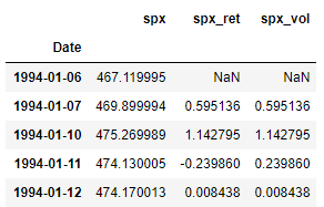
Since this is same code used in the previous parts of this series, the individual lines are not explained in detail here for brevity.
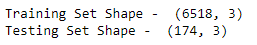
Train-Test Split
We now split the data into train and test sets. Here all the observations on and from 2019–01–01 form the test set, and all the observations before that is the train set.
A word on Stationarity
Stationarity, in the context of time series analysis, means that the statistical properties of a series (mean, variance, etc.) remain fairly constant over time. While fitting statistical models, stationarity in a series is highly desirable. This is due to the face that, if a series is non-stationary, then its distribution will change over time. So, the distribution of data used to train models will be different than the distribution of data for which forecast needs to be generated. Therefore, the quality of forecasts will most likely be poor.
To check for stationarity, we use the ADF (Augmented-Dickey Fuller) Test. It has the following 2 hypothesis:
- Null Hypothesis (H0): Series has a unit root, or it is not stationary.
- Alternate Hypothesis (H1): Series has no unit root, or it is stationary.
The ADF test outputs the test statistic along with the p-value of the statistic. If the p-value of the statistic is less than the confidence levels: 1% (0.01), 5% (0.05) or 10% (0.10) ) then we can reject the Null Hypothesis and call the series stationary.
Stationarity of S&P 500 Returns
Let us use the adfuller() from statsmodels.tsa.stattools package in python to check the stationarity of the series used in this article: S&P 500 Returns ( spx_ret ).
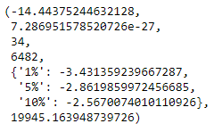
Since, the p-value (2nd value in the tuple returned by the adfuller() function) is much less than any of the confidence levels, we can conclude that the series is stationary. Thus, we can use this series to build models, and use these models to forecast for our test set.
Non Seasonal Models : ARIMA
The non seasonal SARIMA model: ARIMA is an acronym for Auto-Regressive Integrated Moving Average Model. This model is a collection of 3 components:
- AR (Auto-Regressive Component): This component of the ARIMA model is used to capture the dependence of current observation with past observations. The parameter of ARIMA models that control this component is denoted as p.
- I (Integrated): This component of the ARIMA model is used to denote the number of times the series needs to be differenced with lagged versions of itself. Ideally this operation of differencing should be carried out till the series is stationary. The parameter of ARIMA models that control this component is denoted as d.
- MA (Moving Average): This component of the ARIMA model is used to capture the effect of past residuals on the value of the current observation. The parameter of ARIMA models that control this component is denoted as q.
An ARIMA models is usually specified as follows: ARIMA(p, d, q). The parameters p, d, and q represent the AR, I and MA components of the model as described above.
Parameter Selection for ARIMA Models
The following rules are general guidelines that are commonly followed while choosing initial parameters for the ARIMA models.
- p (AR Component): The number of significant lags in the PACF plot of the series is a good stating point for AR component.
- d (I Component): If the series is not stationary and needs to be differenced a certain number of times to remove trend and stationarity, then the number of times this operation is done becomes the order of the Integrated Component.
- q (MA Component): The number of significant lags in the ACF plot of the series is a good stating point for AR component.
Let’s start the model building process by first plotting the ACF and PACF plots for S&P 500 Returns. With these graphs we will estimate the optimal parameters for the ARIMA model.
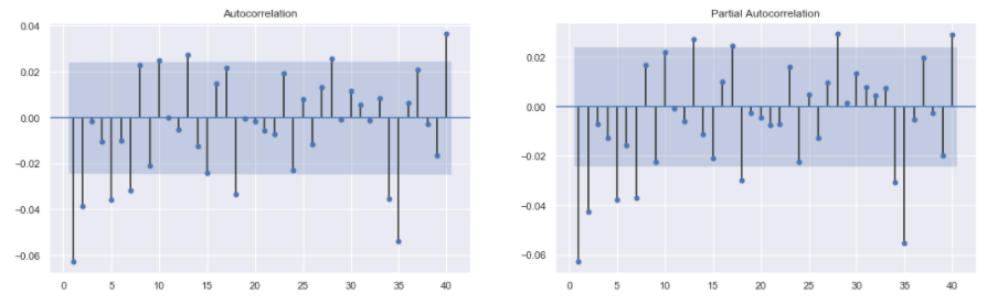
The plot_acf() and plot_pacf() functions are used from the statsmodels.graphics.tsaplots package in python to plot the ACF and PACF plots. The zero = False argument in these functions is used to make sure that the zero-th lag is not plotted. This lag is the input series itself and thus, it will always be perfectly correlated. Hence, including it will not give any new insights. The lags = 40 argument is used to plot ACF and PACF plots for 40 lags in the past.
Note: The input series for the plot_acf() and plot_pacf() functions should be free of any Null values.
The output shows that for both ACF and PACF plots, the first 2 lags seem significant. The significance levels drop significantly after the first 2 lags and spikes back up from 5th lag onward. Thus, a reasonable starting point for the ARIMA parameters is:
- p = 1 or p = 2 (from PACF plot)
- d = 0 (the series was already stationary as proved by the ADF test)
- q = 1 or q = 2 (from ACF plot)
Thus we have a choice between the following models: ARIMA(1, 0, 1), ARIMA(1, 0, 2), ARIMA(2, 0, 1), and ARIMA(2, 0, 2). Just to keep things simple, the ARIMA(1, 0, 1) is built in this series. Since, there is no Integrated component here, we can also call this model ARMA(1, 1).
Fitting ARIMA(1, 0, 1)
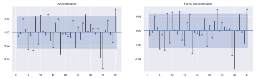
Now we will fit an ARIMA(1, 0, 1) model for S&P 500 returns. After fitting the model, we will plot the ACF and PACF plots of the residuals of this model. If the model is good then the residuals will be similar to random noise (or white noise). This means that a good model will yield residuals that are unpredictable and have no underlying patterns. In terms of ACF and PACF plots, there should be no significant lags for the residuals of a good ARIMA model.
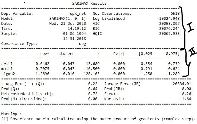
The SARIMAX() function from statsmodels.tsa.statespace.sarimax package in python is used to build the ARIMA(1, 0, 1) model. The training series is passed as the first argument to SARIMAX() function. The next argument is order . This is a tuple representing the (p, d, q) order of the model. In this case the tuple was (1, 0, 1) . The model is defined and stored in the variable model . The fit() method is called on this variable and the fitted model is stored in the variable model_results . The summary() method is called on the model_results variable and is used to display the summary table. Next, the resid method is called on model_results variable to get the residuals. The ACF and PACF plots for the model_results.resid series is then generated.
Summary Table: In the summary table, there are 3 distinct sections (shown in the image above). The first 2 sections are marked in the image. The second column of section I contains some useful metrics that are used to compare different ARIMA models. As a general rule of thumb, the model with higher Log Likelihood or lower IC (AIC, BIC or HQIC) is better, and vice versa. Section II of the summary table gives information about the different coefficients of the AR, and MA components, and the constants used in the model. The coef column contains the actual value of the coefficients, and the P>|Z| column contains the confidence levels. This column indicates whether the coefficients are significant. If the confidence level is set at 5%, then the significant coefficients will have value <0.05 in this column. Therefore, in this case, all the coefficients are clearly significant.
Residuals: If a model is performing well, then the residuals or errors made by the model must not have any underlying pattern in them. If that is the case then the model fails to capture all the information in the data. Thus, a successful model should result in residuals that have no patterns, or the residuals generated in such a case should resemble white noise. This can be checked by making sure that there are no significant lags in the ACF and PACF plots of the residuals. The ACF and PACF plots of the residuals of this model, as seen in the image above, have almost no significant lags. Hence, this model captures all the information reasonably well.
Seasonal Model: SARIMA
The ARIMA model explored above cannot effectively capture the seasonal patterns in the series. For this, we use the SARIMA class of models. SARIMA stands for Seasonal Auto-Regressive Integrated Moving Average model. A SARIMA models is specified as follows: SARIMA(p, d, q)(P, D, Q, m)
Non-Seasonal Parameters:
- p (AR component): Same as the AR component in ARIMA.
- d (I component): Same as the I component in ARIMA. Denotes the number of times successive differencing operation is performed to make the series stationary.
- q (MA component): Same as the MA component in ARIMA.
Seasonal Parameters:
- m (Seasonal Period): This denotes the number of periods in the series after which a seasonal pattern is repeated. It is common to see this parameter also denoted by the letter s.
- P (Seasonal AR component): This parameter captures the effect of past lags on current observations. Unlike p, the past lags are separated from the current lag by multiples of m lags. For eg, if m=12, and P=2, then the current observation is estimated using observations from the 12th lag and 24th lag.
- D (Seasonal I component): This is the number of times seasonal differences need to be calculated in order to make the series stationary. Unlike d, where the differencing was done with successive observations (1st lagged series), here the differencing is done between the series and mth lagged series.
- Q (Seasonal MA Component): This parameter captures the effect of past residuals on current observations. Unlike q, the past lags are separated from the current lag by multiples of m lags. For eg, if m=12, and Q=2, then the current observation is estimated using residuals from the 12th lag and 24th lag.
Parameter Estimation of SARIMA Models
The parameters of the SARIMA(p, d, q)(P, D, Q, m) are estimated using the following general guidelines:
- p: Plot the PACF plot for the series and count the number of significant lags.
- d: The number of successive differencing operations needed to convert the series to stationary.
- q: Plot the ACF plot for the series and count the number of significant lags.
- m: The number of lags after which some seasonal pattern is observed.
- P: Plot the PACF plot again, and observe the number of significant lags separated by multiples of m.
- D: The number of seasonal differences needed to convert the series to stationary.
- Q: Plot the ACF plot again, and observe the number of significant lags separated by multiples of m.
We have already made the ACF and PACF plots for the S&P 500 Returns series. For ease of access, the same image of the plots is displayed below:
Parameter Estimation:
- p = 1, or p = 2 : First 2 lags of PACF are significant.
- d = 0 : No successive differencing was performed in the S&P 500 Returns series.
- q = 1, or q = 2 : First 2 lags of ACF are significant.
- m = 5 : The observations are observed on business days (5 days a week) and there was presence of a seasonal pattern in the decomposition of the series done in part 2 of this series.
- P = 1 : 5th lag is significant in PACF plot.
- D = 0 : There was no seasonal differencing performed here.
- Q = 1, or Q = 2 : 5th and 10th lags are significant in ACF plot.
Using a permutation of all the parameters above we can have 8 different models:
- SARIMA(1, 0, 1)(1, 0, 1, 5)
- SARIMA(1, 0, 1)(1, 0, 2, 5)
- SARIMA(1, 0, 2)(1, 0, 1, 5)
- SARIMA(1, 0, 2)(1, 0, 2, 5)
- SARIMA(2, 0, 1)(1, 0, 1, 5)
- SARIMA(2, 0, 1)(1, 0, 2, 5)
- SARIMA(2, 0, 2)(1, 0, 1, 5)
- SARIMA(2, 0, 2)(1, 0, 2, 5)
Like ARIMA, lets use the simplest one, which is SARIMA(1, 0, 1)(1, 0, 1, 5)
Fitting SARIMA(1, 0, 1)(1, 0, 1, 5)
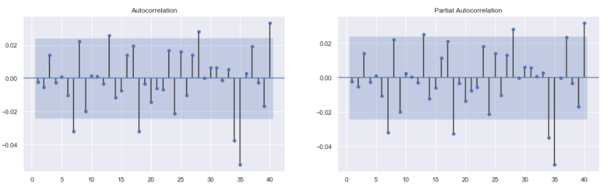
Very similar to fitting the ARIMA(1, 0, 1) model, we will now fit a SARIMA(1, 0, 1)(1, 0, 1, 5) model to S&P 500 Returns. Then using the ACF and PACF plots on the residuals the models performance will be evaluated. If the model is able to capture the information in the data then the residuals should resemble white noise. In other words, the ACF and PACF plots of the residuals should result in no significant lags.
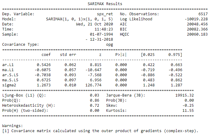
The code used to fit the SARIMA model is almost the same as the one used for ARIMA model. The only difference is the addition of the seasonal_order parameter in the SARIMAX() function. Like ARIMA, here also a SARIMA model is fitted to the S&P 500 Returns series, the summary table is printed out, and the ACF and PACF plots for the residuals are constructed.
The summary table shows that all the coefficients are significant and, the residuals resemble white noise based on the ACF and PACF plots. Thus the model performs well in capturing all the information in the series.
Forecasting using ARIMA and SARIMA
Let us now forecast the S&P 500 Returns using the models that we trained in the previous sections.
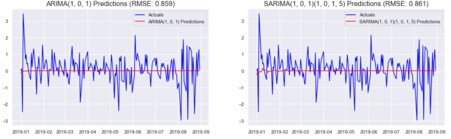
The predict() method is called on the fitted models to generate a series of predictions between the time interval specified by the start and the end parameters of the function. Once we have the predictions, the mean_squared_error() function, from sklearn.metrics, is used to generate the MSE (Mean Squared Error) score for the predictions. sqrt() , A simple square root function from numpy , is then used to generate the RMSE (Root Mean Squared Error) score for the predictions. The predictions are then plotted against the actual observations in the test set to see the performance of the model.
The image above shows that the ARIMA model slightly outperforms the SARIMA model for S&P 500 Returns based on the RMSE score. However, the Log Likelihood, AIC etc. indicate that the SARIMA model outperforms the ARIMA model. The RMSE is calculated over predictions in the test set. On the other hand, the AIC is calculated over the train set. Thus if the priority is to model the train set well, then the model with lower AIC should be preferred, and if the model should perform well on the test set, then RMSE will have greater importance. In this case, we want better predictions, and hence, we will choose the model that performs the best on the test set. Therefore, the final model chosen for S&P 500 Returns is ARIMA(1, 0, 1).
Confidence Intervals
Confidence Intervals give an idea about the margin of error that could be associated with the predictions. They offer unique insights about when, and to what extent are the predictions stable. That is why they are important while making business decisions based on the forecasts. Now let’s generate confidence intervals for the ARIMA(1, 0, 1) model from above.
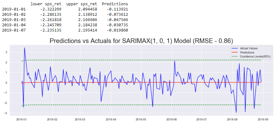
First we use the get_forecast() function on the fitted model: model_results , and store the output in the variable forecasts . The function takes in an integer number of periods for which the forecasts need to be generated. In this case, we specify the number of periods in the test set as the argument. Next, the conf_int() function is called on the forecasts object. This function takes in argument alpha which controls the confidence level. alpha = 0.05 indicates that we have 95% confidence in observing the predictions between the intervals shown in green in the image. We then generate the predictions from the model using the predict() method as before. The first few rows of the forecasts_df is displayed for better visualization of the data. Finally, the forecasts, and confidence intervals are plotted against the actual values of the S&P 500 Returns.
Conclusions
In this article we looked at the SARIMA class of models. We used these models to fit S&P 500 Returns series. Then we used these models to get confidence intervals for our predictions. However, the confidence intervals generated were constant and did not offer any significant insight on our model’s predictions.
In the image above, it is clear that there are regions where the model had reasonably accurate predictions and there were regions where the predictions were off by a bigger margin. The confidence intervals should reflect these changes in prediction accuracy. To do this, we will use a GARCH model on top of the ARIMA model from this article. So the next article will first introduce the GARCH model, and the one after that covers ARIMA+GARCH model to fit S&P 500 Returns.
Links to other parts of this series
- Statistical Modeling of Time Series Data Part 1: Preprocessing
- Statistical Modeling of Time Series Data Part 2: Exploratory Data Analysis
- Statistical Modeling of Time Series Data Part 3: Forecasting Stationary Time Series using SARIMA
- Statistical Modeling of Time Series Data Part 4: Forecasting Volatility using GARCH
- Statistical Modeling of Time Series Data Part 5: ARMA+GARCH model for Time Series Forecasting.
- Statistical Modeling of Time Series Data Part 6: Forecasting Non — Stationary Time Series using ARMA
References
[1] 365DataScience Course on Time Series Analysis
[2] machinelearningmastery blogs on Time Series Analysis
[3] Wikipedia articles on SARIMA class of models
[4] Tamara Louie: Applying Statistical Modeling & Machine Learning to Perform Time-Series Forecasting
[5] Forecasting: Principles and Practice by Rob J Hyndman and George Athanasopoulos
[6] A Gentle Introduction to Handling a Non-Stationary Time Series in Python from Analytics Vidhya
Statistical Modeling of Time Series Data Part 3: Forecasting Stationary Time Series using SARIMA was originally published in Towards AI on Medium, where people are continuing the conversation by highlighting and responding to this story.
Published via Towards AI
Towards AI Academy
We Build Enterprise-Grade AI. We'll Teach You to Master It Too.
15 engineers. 100,000+ students. Towards AI Academy teaches what actually survives production.
Start free — no commitment:
→ 6-Day Agentic AI Engineering Email Guide — one practical lesson per day
→ Agents Architecture Cheatsheet — 3 years of architecture decisions in 6 pages
Our courses:
→ AI Engineering Certification — 90+ lessons from project selection to deployed product. The most comprehensive practical LLM course out there.
→ Agent Engineering Course — Hands on with production agent architectures, memory, routing, and eval frameworks — built from real enterprise engagements.
→ AI for Work — Understand, evaluate, and apply AI for complex work tasks.
Note: Article content contains the views of the contributing authors and not Towards AI.
Related posts


")
Recent Posts


")

