LDA vs. PCA

Last Updated on January 26, 2022 by Editorial Team

Author(s): Pranavi Duvva

 

A precise overview on how similar or dissimilar is the Linear Discriminant Analysis dimensionality reduction technique from the Principal Component Analysis

This is the second part of my earlier article which is The power of Eigenvectors and Eigenvalues in dimensionality reduction techniques such as PCA.

In this article, I will start with a brief explanation of the differences between LDA and PCA. Let’s then deep dive into the working of the Linear discriminant analysis and unravel the mystery, How it achieves classification of the data along with the dimensionality reduction.

Introduction

LDA vs. PCA

Linear discriminant analysis is very similar to PCA both look for linear combinations of the features which best explain the data.

The main difference is that the Linear discriminant analysis is a supervised dimensionality reduction technique that also achieves classification of the data simultaneously.

LDA focuses on finding a feature subspace that maximizes the separability between the groups.

While Principal component analysis is an unsupervised Dimensionality reduction technique, it ignores the class label.

PCA focuses on capturing the direction of maximum variation in the data set.

LDA and PCA both form a new set of components.

The PC1 the first principal component formed by PCA will account for maximum variation in the data.PC2 does the second-best job in capturing maximum variation and so on.

The LD1 the first new axes created by Linear Discriminant Analysis will account for capturing most variation between the groups or categories and then comes LD2 and so on.

Note: In, LDA The target dependent variable can have binary or multiclass labels.

Working of Linear Discriminant Analysis

Let’s understand the working of the Linear Discriminant Analysis with the help of an example.

Imagine you have a credit card loan dataset with a target label consisting of two classes defaulter and non-defaulter.

Class‘ 1’ is the defaulter and class ‘0’ is the non-defaulter.

Understanding a basic 1-D and 2-D graph before proceeding on to LDA projection

When you have just one attribute say the credit score the graph would be a 1-D graph which is a number line.

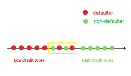
With just one attribute, although we were able to separate the categories certain points have been over-lapped due to no specific cut-off point. In reality, there could be many such overlapped data points when there is a large number of observations in the data set.

Let’s see what happens when we have two attributes, are we able to classify better?

Considering another attribute annual income along with the credit score.

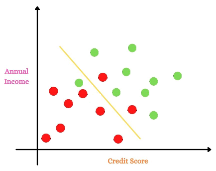
Adding another feature, we were able to reduce the overlapping than the earlier case with a single attribute. But when we work on large data sets with many features and observations, there would still be a lot many overlapped points left.

Something interesting, we noticed is adding features we were able to reduce the number of overlapped points and distinguish better. But this becomes extremely difficult to visualize when we have high dimension dataset.

This is where the implementation of LDA plays a crucial role.

How does LDA project the data?

Linear Discriminant Analysis projects the data points onto new axes such that these new components maximize the separability among categories while keeping the variation within each of the categories at a minimum value.

Let us now understand in detail how LDA projects the data points.

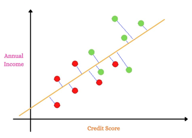
1.LDA uses information from both the attributes and projects the data onto the new axes.

2.It projects the data points in such a way that it satisfies the criteria of maximum separation between groups and minimum variation within groups simultaneously.

Step 1:

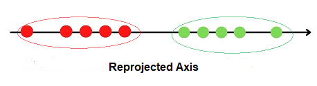
The projected points and the new axes

Step-2

Criterion LDA applies to the projected points is as follows.

1.It maximizes the distance between the means of each category.

2. It minimizes the variation or scatter within each category represented by s²

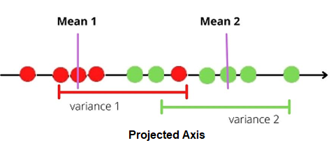
Let the mean of the category 1 defaulter be mean 1 and mean 2 be the mean of the category non-defaulter.

Similarly,

S1² be the scatter of the first category and

S2² be the scatter of the second category.

It now calculates the formula.

(mean1-mean2)²/(S1²+S2²)

Note: Numerator is squared to avoid negative values.

Let mean1-mean2 be represented by d.

The formula will now be.

d²/(S1²+S2²)

Note: Ideally, the Larger, the numerator greater, the separation between groups. While smaller the denominator less variance within the groups.

How does LDA work when there are more than two categories?

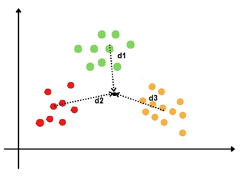
When there are more than two categories, LDA calculates the central point of all the categories and the distance between the central points of each category to that point.

It then projects the data onto the new axes in such a way that there is a maximum separation between the groups and minimum variation within the groups.

The formula will now be.

(d1²+d2²+d3²)/(s1²+S2²+S3²)

and now the curious part…

How does LDA make predictions?

Linear Discriminant Analysis uses Baye’s theorem to estimate the probabilities.

It first calculates the prior probabilities from the given data set. With the help of these prior probabilities, it calculates the posterior probabilities using Baye’s theorem.

From Bayes Theorem we know that.

P(A|B)=P(B|A)*P(A)/P(B)

where A, B are events and P(B) is not equal to zero

Assume we have three classes class 0, class 1, class 2 in the data set.

step 1

LDA calculates the prior probabilities of each of the classes P(y=0), P(y=1), P(y=2) of the data set.

Next, it calculates the conditional probabilities of the observations.

step 2

let us consider an observation x.

P(x|y=0),P(x|y=1),P(x|y=2) represent the likelihood functions.

step 3

LDA now calculates the Posterior probabilities to make predictions.

P(y=0|x)=P(x|y=0)*P(y=0)/P(x)

P(y=1|x)=P(x|y=1)*P(y=1)/P(x)

P(y=2|x)=P(x|y=2)*P(y=2)/P(x)

The general equation for a set of ‘c’ classes

Let y1, y2,.., yc be the set of ‘c’ classes and consider i=1,2,..,c.

P(x|yi) will represent the likelihood function or the conditional probability.

P(yi) will be the prior probability of each class in the data set. Which is nothing but the ratio of the number of observations in that particular class to the total number of observations in all the classes.

The posterior probability will be Likelihood*Prior/Evidence.

P(y=yi|x)=P(x|y=yi)*P(yi)/P(x)

Assumptions of Linear Discriminant Analysis

There are certain assumptions Linear Discriminant Analysis makes on the data set they are.

Assumption 1

LDA assumes that the independent variables are normally distributed for each of the categories.

Assumption 2

Homoscedascity

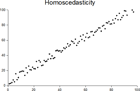
LDA assumes the independent variables have equal variances and covariances across all the categories. This can be tested with Box’s M statistic.

In simple words, The assumption states that the variance across all variables for the categories in the data set say when y=0, y=1 has to be equal, and also the covariance between the variables has to be equal.

This assumption helps the Linear Discriminant Analysis to create the linear decision boundary between the categories.

Assumption 3

Multicollinearity

The performance of prediction can decrease with the increased correlation between the independent variables.

Note: Studies show that LDA is robust to slight violations of these assumptions.

What happens when the second assumption fails?

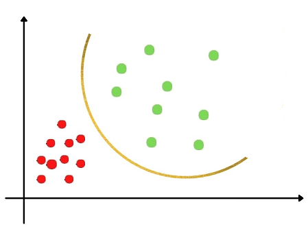
When this assumption fails, There is huge variation between the classes in the data set and the other variant of Discriminant analysis is used which is the Quadratic Discriminant Analysis (QDA).

In Quadratic Discriminant Analysis, The mathematical function which separates the categories will now be quadratic and not linear to achieve classification.

Applications of LDA

1. LDA is most widely used in pattern recognition tasks. For example, analyzing customer behavior patterns based on attributes.
2. Image recognition, LDA can distinguish between categories. For example Faces and not faces, objects and not objects.
3. In the medical field, To classify patients into different groups based on symptoms for a particular disease.

Conclusion

This article has explained the differences between the two commonly used dimensionality reduction techniques Principal Component Analysis and Linear Discriminant Analysis. It then covered the working principle of the Linear Discriminant analysis and how it achieves classification along with dimensionality reduction.

Hope you enjoyed reading this article!

Please feel free to check my other articles on pranaviduvva at medium.

Thanks for reading!

References

1. https://scikit-learn.org/stable/modules/lda_qda.html
2. https://en.wikipedia.org/wiki/Bayes%27_theorem
3. https://en.wikipedia.org/wiki/Linear_discriminant_analysis
4. Statquest video on LDA.

---

LDA vs. PCA was originally published in Towards AI on Medium, where people are continuing the conversation by highlighting and responding to this story.

Published via Towards AI