Efficient Pandas: Using Chunksize for Large Datasets

Last Updated on December 10, 2020 by Editorial Team

Author(s): Lawrence Alaso Krukrubo 

Exploring large data sets efficiently using Pandas

Data Science professionals often encounter very large data sets with hundreds of dimensions and millions of observations. There are multiple ways to handle large data sets. We all know about the distributed file systems like Hadoop and Spark for handling big data by parallelizing across multiple worker nodes in a cluster. But for this article, we shall use the pandas chunksize attribute or get_chunk() function.

Imagine for a second that you’re working on a new movie set and you’d like to know:-

1. What’s the most common movie rating from 0.5 to 5.0

2. What’s the average movie rating for most movies produced.

To answer these questions, first, we need to find a data set that contains movie ratings for tens of thousands of movies. Thanks to Grouplens for providing the Movielens data set, which contains over 20 million movie ratings by over 138,000 users, covering over 27,000 different movies.

This is a large data set used for building Recommender Systems, And it’s precisely what we need. So let’s extract it using wget. I’m working in Colab, but any notebook or IDE is fine.

!wget -O moviedataset.zip https://s3-api.us-geo.objectstorage.softlayer.net/cf-courses-data/CognitiveClass/ML0101ENv3/labs/moviedataset.zip

print('unziping ...')

!unzip -o -j moviedataset.zip

Unzipping the folder displays 4 CSV files:

links.csv

movies.csv

ratings.csv

tags.csv

Our interest is on the ratings.csv data set, which contains over 20 million movie ratings for over 27,000 movies.

# First let's import a few libraries
import pandas as pd
import matplotlib.pyplot as plt

Let’s take a peek at the ratings.csv file

ratings_df = pd.read_csv('ratings.csv')
print(ratings_df.shape)
>>
  (22884377, 4)

As expected, The ratings_df data frame has over twenty-two million rows. This is a lot of data for our computer’s memory to handle. To make computations on this data set, it’s efficient to process the data set in chunks, one after another. In sort of a lazy fashion, using an iterator object.

Please note, we don’t need to read in the entire file. We could simply view the first five rows using the head() function like this:

pd.read_csv('ratings.csv').head()

It’ s important to talk about iterable objects and iterators at this point…

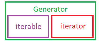
An iterable is an object that has an associated iter() method. Once this iter() method is applied to an iterable, an iterator object is created. Under the hood, this is what a for loop is doing, it takes an iterable like a list, string or tuple, and applies an iter() method and creates an iterator and iterates through it. An iterable also has the __get_item__() method that makes it possible to extract elements from it using the square brackets.

See an example below, converting an iterable to an iterator object.

# x below is a list. Which is an iterable object.
x = [1, 2, 3, 'hello', 5, 7]

# passing x to the iter() method converts it to an iterator.
y = iter(x)

# Checking type(y)
print(type(y))
>>
<class 'list_iterator'>

The object returned by calling the pd.read_csv() function on a file is an iterable object. Meaning it has the __get_item__() method and the associated iter() method. However, passing a data frame to an iter() method creates a map object.

df = pd.read_csv('movies.csv').head()

# Let's pass the data frame df, to the iter() method
df1 = iter(df)

print(type(df1))
>>
<class 'map'>

An iterator is defined as an object that has an associated next() method that produces consecutive values.

To create an iterator from an iterable, all we need to do is use the function iter() and pass it the iterable. Then once we have the iterator defined, we pass it to the next() method and this returns the first value. calling next() again returns the next value and so on… Until there are no more values to return and then it throws us a StopIterationError.

x = [1, 2, 3]

x = iter(x)  # Converting to an iterator object

# Let’s call the next function on x using a for loop
for i in range(4): print(next(x))
>>
1
2
3
StopIterationError
# Error is displayed if next is called after all items have been printed out from an iterator object

Note that the terms function and method have been used interchangeably here. Generally, they mean the same thing. Just that a method is usually applied on an object like the head() method on a data frame, while a function usually takes in an argument like the print() function.

If you’d like to find out about python comprehensions and generators see this link to my notebook on Github. It’s not necessary for this article.

Ok. let’s get back to the ratings_df data frame. We want to answer two questions:

1. What’s the most common movie rating from 0.5 to 5.0

2. What’s the average movie rating for most movies.

Let’s check the memory consumption of the ratings_df data frame

ratings_memory = ratings_df.memory_usage().sum()

# Let's print out the memory consumption
print('Total Current memory is-', ratings_memory,'Bytes.')

# Finally, let's see the memory usage of each dimension.
ratings_df.memory_usage()
>>
Total Current memory is- 732300192 Bytes.

Index              128
userId       183075016
movieId      183075016
rating       183075016
timestamp    183075016
dtype: int64

We can see that the total memory consumption of this data set is over 732.3 million bytes… Wow.

Since we’re interested in the ratings, let’s get the different rating keys on the scale, from 0.5 to 5.0

# Let's get a list of the rating scale or keys
rate_keys = list(ratings_df['rating'].unique())

# let's sort the ratings keys from highest to lowest.
rate_keys = sorted(rate_keys, reverse=True) 
 
print(rate_keys)
>>
  [5.0, 4.5, 4.0, 3.5, 3.0, 2.5, 2.0, 1.5, 1.0, 0.5]

We now know our rating scale. Next, is to find a way to get the number of ratings for each key on the scale. Yet due to the memory size, we should read the data set in chunks and perform vectorized operations on each chunk. Avoiding loops except necessary.

Our first goal is to count the number of movie ratings per rating key. Out of the 22 million-plus ratings, how many ratings does each key hold? Answering this question automatically answers our first question:-

Question One:

1. What’s the most common movie rating from 0.5 to 5.0

let’s create a dictionary whose keys are the unique rating keys using a simple for loop. Then we assign each key to value zero.

ratings_dict = {}
for i in rate_keys: ratings_dict[i] = 0

ratings_dict
>>

{0.5: 0,  1.0: 0,  1.5: 0,  2.0: 0,  2.5: 0,  3.0: 0,  3.5: 0,  4.0: 0,  4.5: 0,  5.0: 0}

Next, we use the python enumerate() function, pass the pd.read_csv() function as its first argument, then within the read_csv() function, we specify chunksize = 1000000, to read chunks of one million rows of data at a time.

We start the enumerate() function index at 1, passing start=1 as its second argument. So that we can compute the average number of bytes processed for each chunk using the index. Then we use a simple for loop on the rating keys and extract the number of ratings per key, for each chunk and sum these up for each key in the ratings_dict

The final ratings_dict will contain each rating key as keys and total ratings per key as values.

Using chunksize attribute we can see that :
Total number of chunks: 23
Average bytes per chunk: 31.8 million bytes

This means we processed about 32 million bytes of data per chunk as against the 732 million bytes if we had worked on the full data frame at once. This is computing and memory-efficient, albeit through lazy iterations of the data frame.

There are 23 chunks because we took 1 million rows from the data set at a time and there are 22.8 million rows. So that means the 23rd chunk had the final 0.8 million rows of data.

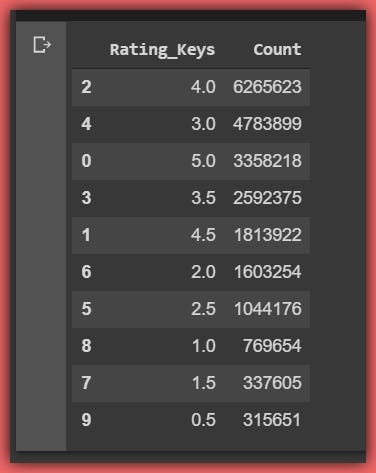
We can also see our ratings_dict below complete with each rating key and the total number of ratings per key

{5.0: 3358218, 4.5: 1813922, 4.0: 6265623, 3.5: 2592375, 3.0: 4783899, 2.5: 1044176, 2.0: 1603254, 1.5: 337605, 1.0: 769654, 0.5: 315651}

Note that By specifying chunksize in read_csv, the return value will be an iterable object of type TextFileReader .Specifying iterator=True will also return the TextFileReader object:

# Example of passing chunksize to read_csv
reader = pd.read_csv(’some_data.csv’, chunksize=100)
# Above code reads first 100 rows, if you run it in a loop, it reads the next 100 and so on

# Example of iterator=True. Note iterator=False by default.
reader = pd.read_csv('some_data.csv', iterator=True)
reader.get_chunk(100)
This gets the first 100 rows, running through a loop gets the next 100 rows and so on.

# Both chunksize=100 and reader.get_chunk(100) return same TextFileReader object.

This shows that the chunksize acts just like the next() function of an iterator, in the sense that an iterator uses the next() function to get its’ next element, while the get_chunksize() function grabs the next specified number of rows of data from the data frame, which is similar to an iterator.

Before moving on, let’s confirm we got the complete ratings from the exercise we did above. Total ratings should be equal to the number of rows in the ratings_df.

sum(list(ratings_dict.values())) == len(ratings_df)
>>
True

Let’s finally answer question one by selecting the key/value pair from ratings_dict that has the max value.

# We use the operator module to easily get the max and min values
import operator
max(ratings_dict.items(), key=operator.itemgetter(1))

>>
  (4.0, 6265623)

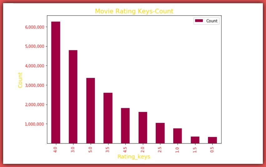
We can see that the rating key with the highest rating value is 4.0 with a value of 6,265,623 movie ratings.

Thus, the most common movie rating from 0.5 to 5.0 is 4.0

Let’s visualize the plot of rating keys and values from max to min.

Let’s create a data frame (ratings_dict_df) from the ratings_dict by simply casting each value to a list and passing the ratings_dict to the pandas DataFrame() function. Then we sort the data frame by Count descending.

Question Two:

2. What’s the average movie rating for most movies.

To answer this, we need to calculate the Weighted-Average of the distribution.

This simply means we multiply each rating key by the number of times it was rated and we add them all together and divide by the total number of ratings.

# First we find the sum of the product of rate keys and corresponding values.
product = sum((ratings_dict_df.Rating_Keys * ratings_dict_df.Count))

# Let's divide product by total ratings.
weighted_average = product / len(ratings_df)

# Then we display the weighted-average below.
weighted_average
>>
  3.5260770044122243

So to answer question two, we can say

The average movie rating from 0.5 to 5.0 is 3.5.

It’s pretty encouraging that on a scale of 5.0, most movies have a rating of 4.0 and an average rating of 3.5… Hmm, Is anyone thinking of movie production?

If you’re like most people I know, the next logical question is:-

Hey Lawrence, what’s the chance that my movie would at least be rated average?

To find out what percentage of movies are rated at least average, we would compute the Relative-frequency percentage distribution of the ratings.

This simply means what percentage of movie ratings does each rating key hold?

Let’s add a percentage column to the ratings_dict_df using apply and lambda.

ratings_dict_df['Percent'] = ratings_dict_df['Count'].apply(lambda x: (x / (len(ratings_df)) * 100))

ratings_dict_df
>>

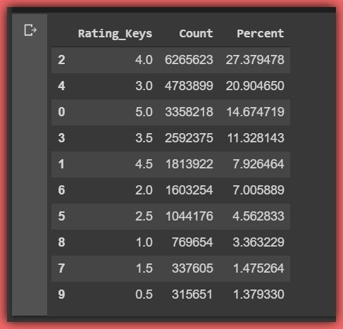
Therefore to find the percentage of movies that are rated at least average (3.5), we simply sum the percentages of movie keys 3.5 to 5.0.

sum(ratings_dict_df[ratings_dict_df.Rating_Keys >= 3.5]['Percent'])
>>
  61.308804692389046

Findings:

From these exercises, we can infer that on a scale of 5.0, most movies are rated 4.0 and the average rating for movies is 3.5 and finally, over 61.3% of all movies produced have a rating of at least 3.5.

Conclusion:

We’ve seen how we can handle large data sets using pandas chunksize attribute, albeit in a lazy fashion chunk after chunk.

The merits are arguably efficient memory usage and computational efficiency. While demerits include computing time and possible use of for loops. It’s important to state that applying vectorised operations to each chunk can greatly speed up computing time.

Thanks for your time.

P.S See a link to the notebook for this article in Github.

Bio: Lawrence Krukrubo is a Data Specialist at Tech Layer Africa, passionate about fair and explainable AI and Data Science. Lawrence is certified by IBM as an Advanced-Data Science Professional. He loves to contribute to open-source projects and has written several insightful articles on Data Science and AI. Lawrence holds a BSc in Banking and Finance and pursuing his Masters in Artificial Intelligence and Data Analytics at Teesside, Middlesbrough U.K.

---

Efficient Pandas: Using Chunksize for Large Datasets was originally published in Towards AI on Medium, where people are continuing the conversation by highlighting and responding to this story.

Published via Towards AI