Data Science Evaluation Metrics — Unravel Algorithms for Regression [Part 2]

Last Updated on January 6, 2023 by Editorial Team

Author(s): Maximilian Stäbler

Data Science

Error Formulas Data Science Evaluation Metrics — Unravel Algorithms for Regression [Part 2]

Lessons learned about evaluation metrics for classification tasks.

Before we get started: This post deals exclusively with evaluation metrics for regressions! I have already written another post (first part) about methods for determining the quality of classification problems. That article can be opened here.

Now that this has been clarified let’s turn to the second and remaining method from the field of supervised learning applications. Accordingly, we will again use labeled data sets to predict continuous target variables (y) with the help of different algorithms.
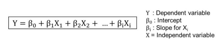
Briefly, the goal of the regression model is to build a mathematical equation that defines y as a function of the x variables. Next, this equation can be used to predict the outcome (y) on the basis of new values of the predictor variables (x). The simplest and, at the same time, the best-known form of regression is linear regression. Every student has worked with the formula during their school years. The picture below shows the formula for multiple regression:

As in Part 1 of this series of articles, however, we will not focus on the various regression algorithms or their advantages and disadvantages, but on how to evaluate a regression result.
The most commonly used metric here is the so-called error. The error is easy to implement and even easier to understand. Basically, you simply compare the predicted value with the real (true) value and calculate the difference. All of these differences are so-called residuals! Residuals in a statistical or machine learning model are, therefore, the differences between observed and predicted values of data. They are a diagnostic measure used when assessing the quality of a model.

Residuals — Why should I care?

In general, one should ALWAYS take a look at the residual plot because, with the correct interpretation, numerous deficiencies and problems of the algorithm used are illustrated there. Here is an overview: (a detailed description of the importance of the residuals can be read here)

— The quality of the model can be assessed by looking at the size of the residuals and any patterning of the residuals.
 — For a perfect model, all residuals would be 0. The further the residuals are from 0, the less accurate the model is. In the case of linear regression, the larger the sum of squared residuals (Mean squared error — explained later), the smaller the R-squared statistic, all else being equal.
 — If the average residual is not 0, it means that the model is systematically biased (i.e., consistently over-or under-predicts).
 — If the residuals contain patterns, it means that the model is qualitatively incorrect because it cannot explain the property of the data. The existence of patterns invalidates most statistical tests.

As in the first part, the corresponding notebook can be cloned on my Github account. All datasets used are also included there.

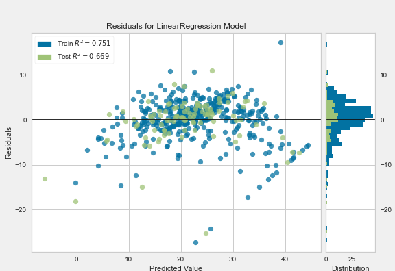
Before we look at the residuals plot, I would like to remind you that residuals are nothing else than the difference between the real value and the model predicted by our model! With this in mind, let’s now look at the residual plot of our linear regression on the known data set (Boston Housing Data).
The goal here is to predict the average value of a property based on its characteristics. Although we have a non-optimized model, we can see an approximately random distribution of the residuals. Generally, a good sign! What should give us something to think about is the slightly upward shifted mean value of the residuals, which can also be seen in the histogram on the right side. There are no patterns to be seen. So we can say that our model is not bad at all but definitely needs some fine-tuning to fix the constant overestimation of the property value.

Ok, I understood how residuals work — what else can be used?

Very good question, the answer to which will please some readers and disappoint some:
There are not as many different methods or approaches to evaluating the model in regression as there are in classification. There, one could find an indiviudellen analysis approach for each model with the Confusion Matrix or most diverse ROC Plots in many different ways.
In a regression task, on the other hand, most of the metrics are based on the residuals presented and only aggregate them in different ways. Why this is so is in the nature of regression:
You predict a value for a particular set of covariates and compare that to the true value. There are no categorical variables here, only the ability to calculate how wrong the prediction is.

Therefore, people who don’t want to remember numerous different methods may be happy here, and people who like to have different approaches to evaluation at hand may be a bit disappointed at this point. For the latter, however, the following applies as always: The approaches presented here in no way constitute a complete overview of all metrics for evaluating regressions! Only the most common metrics are presented.

Variations of the residuals are, for example, the absolute error (absolute values of the deviation), the mean absolute error (mean of the absolute error values), the mean squared error (squared error), the root mean squared error (square root of the mean squared error) and R-squared.

Before we implement these in an example, it is worth taking a look at the individual formulas. You can see that the metrics build on each other, and the residuals form the basis for the calculation of each of these metrics.

For the notation:

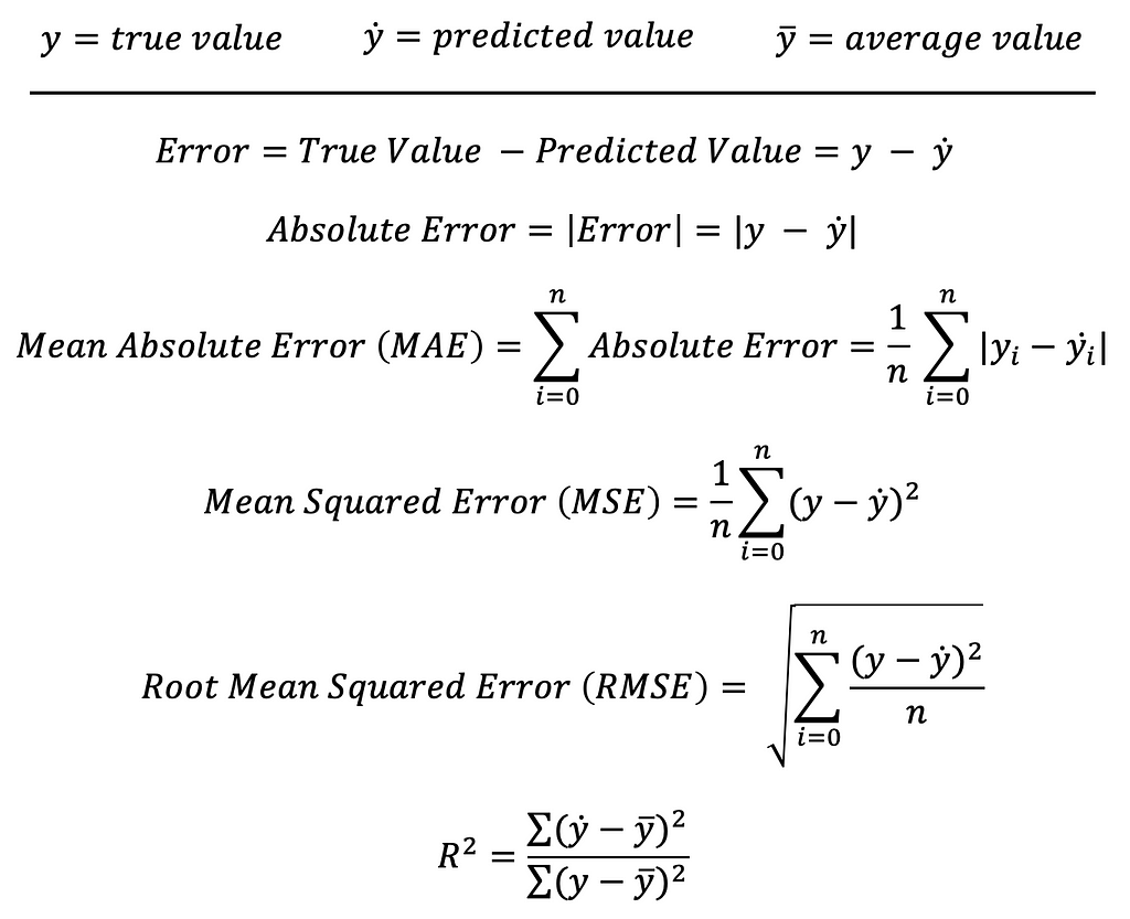
In my opinion, the formulas of the individual metrics are very easy to understand — I hope you see it the same way. Each of these metrics can be the most appropriate in certain applications. However, it must be clearly stated that the MSE, RMSE, and R-squared are the best known and the most commonly used metrics. For this reason, I would like to explain these three in more detail and say what advantages they can offer.

MSE

MSE ensures by squaring that the negative values do not offset the positive ones. The smaller the MSE, the better the model fits the data. The MSE has the units squared of whatever is plotted on the vertical axis. As you can see, as a result of the squaring, it assigns more weight to the bigger errors. The algorithm then continues to add them up and average them. If you are worried about the outliers, this is the number to look at. Keep in mind and it’s not in the same unit as our dependent value.

RMSE

The Root Mean Squared Error (RMSE) is just the square root of the mean square error. That is probably the most easily interpreted statistic since it has the same units as the quantity plotted on the vertical axis. The RMSE is directly interpretable in terms of measurement units, and so is a better measure of goodness of fit than a correlation coefficient. One can compare the RMSE to observed variation in measurements of a typical point. The two should be similar for a reasonable fit.

R-squared

The coefficient of determination of the regression R-squared, also the empirical coefficient of determination, is a dimensionless measure that expresses the portion of the variability in the measured values of the dependent variable, which is “explained” by the linear model. Given the sum-of-squares decomposition, the coefficient of determination of the regression is defined as the ratio of the sum-of-squares explained by the regression to the total sum-of-squares.
R-squared has the useful property that its scale is intuitive: it ranges from zero to one, with zero indicating that the proposed model does not improve prediction over the mean model and one indicating perfect prediction. Improvement in the regression model results in proportional increases in R-squared.
One pitfall of R-squared is that it can only increase as predictors are added to the regression model. This increase is artificial when predictors are not actually improving the model’s fit.

Metrics in action

To compare the metrics, we will compare a Support Vector Regression with a Linear Regression and decide based on the values which method gives better results.
Important: There is no emphasis on the optimization of the individual methods. Simply the default settings are used.

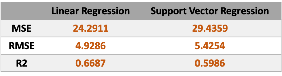
We can see that our linear regression model performs better than SVR in every metric. The decision of which model to use in further steps is therefore not difficult.

Summary

To conclude this article, I would like to summarize the most important points once again:

In contrast to classification tasks, regressions do not have so many different metrics that can be used to evaluate different models.
The most common metrics are MSE, RMSE, and R2.
My personal favorite is R2, simply because the interpretation is intuitive, and it makes comparing different models very easy.

I hope I could give a deeper insight into the evaluation metrics for classification and regression tasks with these two posts.

Thank you very much for your attention!

Here is some more useful and deeper information:

Regression essentials
R squared explained
MSE and RMSE

---

Data Science Evaluation Metrics — Unravel Algorithms for Regression [Part 2] was originally published in Towards AI on Medium, where people are continuing the conversation by highlighting and responding to this story.

Published via Towards AI