Demystifying Principal Component Analysis

Last Updated on July 20, 2020 by Editorial Team

Author(s): Abhijit Roy

Data Science

Data visualization has always been an essential part of any machine learning operation. It helps to get a very clear intuition about the distribution of data, which in turn helps us to decide which model is best for the problem, we are dealing with.

Currently, with the advancement of machine learning, we more often need to deal with large datasets. The datasets are having a large number of features, and can only be visualized using a large feature space. Now, we can only visualize 2-dimensional planes but, visualization of data is also seems pretty necessary, as we saw in our discussion above. This is where Principal Component Analysis comes in.

Principal Component Analysis, or PCA, is a dimensionality-reduction method that is often used to reduce the dimensionality of large data sets, by transforming a large set of variables into a smaller one that still contains most of the information in the large set.

In simple words, it performs dimensionality reduction, i.e., it takes in large datasets with a large number of features and produces a dataset with a lower number of features(as we specify), losing as minimum information as possible.

Now, we need to be clear about a few things.

1. Principle Component Analysis is an Unsupervised technique.
2. If we pass a dataset with 5 features say age, height, weight, IQ, and Gender through PCA and tell it to represent using 2 features, PCA will give us two components, Principle Component 1 and Principle Component 2, these are not any specific features from our 5 initial features, they are combinations of the 5 features that hold maximum information.
3. In a dataset, if we separately view each feature, we will see something like this.

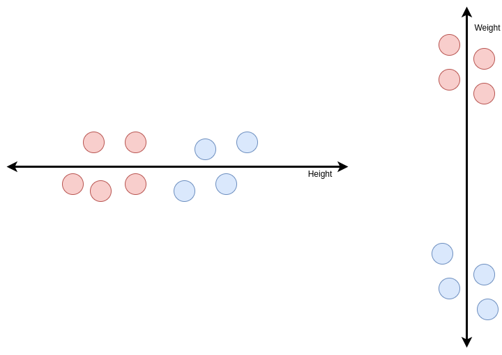
If we view the above diagram and regard the red ball to be class 1 and the blue ones to be class 2, we can see the two classes can be divided based on the features. This character of the features helps a model to segregate between two classes based on the behavior of features. Though we can see for ‘weight’ feature the classes are better divided than the ‘height’ feature. We can say that because we can see for the ‘weights’ the distance between the two classes is more.

This concept is reflected by the Variance of the feature. Variance is given by:

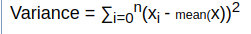
So, it is the summation of the square of the distance from the mean. The more the points are distant more is the variance. So, Weight here has more variance than height. This variance can be used to depict and compare how much information a particular feature provides a model about the distribution of data. More the variance more information is provided.

A theoretical Intuition

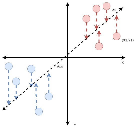
This diagram exactly describes the Principal Component Analysis. Say, we have two features X and Y. We distribute the points on a 2- Dimensional plane, each point can be represented by a tuple (X1, Y1) where they are the values of the features. Now, we want to represent this using only 1 component. So need to find an Axis as shown in the figure, and take the projection of the points located on the XY plane on the Axis. Now the projection can be represented by a single value Z1 as the Axis is 1 Dimensional. The criteria of the axis for suiting our purpose is that the variance of the points for that axis has to be maximum i.e, if we choose any other axis, project the points on it, and find the variance, the value should not be greater than the present value.

But now, as we did a dimension reduction, we will lose some information. Our goal is to minimize information loss. Now, if we have 10 Dimensional Data and we reduce its dimension to 2, it may look something like this.

To, summarize we try to find the best possible axes where the variance along the axes are maximum, then we take the projection of the n-dimensional points on the plane formed by our axes for dimensionality reduction.

An issue we need to address here is, sometimes we may not be able to hold much of the information using the components of PCA. Even though we look for the best axes with maximum variance, still it's not possible to trap full information in our components. In those cases, we should not depend fully on PCA to judge our data as it may miss important intuitions about the data. It is said that if the n components of PCA together cannot capture at least 85% of the information, we should not depend on the results of PCA.

Now, let’s go for the Mathematical Intuition.

The Maths Behind PCA

Principal Component Analysis depends on linear algebra. For this, we must have a very clear idea about the Eigen Vectors and Eigen Values.

So, What are Eigen Vectors and Eigen Values?

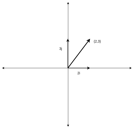
We all know a point (2,3), can be represented as a vector as 2i + 3j. We normally use i and j as the units to represent every vector in our plane. They are called the basis. But, now if someone wants to use different vectors as their basis, or in other words, someone wants to use some other vectors to represent all the vectors, instead of i,j.

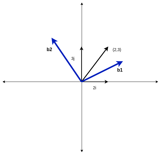
Suppose we want b1 and b2 to be our basis. So, how should we correlate between the two systems?

Now, we will try to see what actually b1 and b2 mean in our system.

Say, we find b1=2i+j and b2=-1i+1j

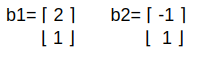
They are 1x 2 matrices or 2D vectors. Sorry, I did not actually find a proper editor, anyways let's continue.

So, we can represent our basis with respect to i and j in this way. Now, what a vector in the b1b2 system means in the ij system.

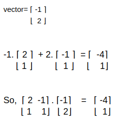
Be aware of the fact that I have written the vectors as a 1 x 2 matrix due to the editor problem. For application, we need to find the transpose of the 1 x 2 matrix to obtain the 2D vector and then perform the multiplication. By the [x y] I mean to represent a vector xi+yj.

So, say we need to convert vector [-1, 2] in the b1b2 system, from the b1b2 system to the ij system we need to find the product of the vector [-1 2] with the matrix given.

Now, it turns out if we pick any vector from the b1b2 system and multiply with this vector we find its corresponding representation in the ij system.

Similarly, we find the Inverse of this matrix. We will obtain,

If we multiply any vector from our ij plane with this matrix we will obtain its corresponding vector on the b1b2 plane.

If we start picking up vectors from the ij plane and multiplying with this matrix, we will obtain a vector in the b1b2 plane for every vector in the ij plane. Thus, we can convert the whole ij plane into b1b2 plane. This is called transformation.

It turns out that, the way a transformation changes the basis of a system, it will change any vector of the system in the same way, i.e, if a transforms scales the basis vectors by 2 it will have the similar effect on the other vectors of that system also, as every vector of a system, depends on the basis vector for representation. So, we will check the changes of the transformation on the basis only to understand clearly.

There are various kinds of transformations, for example, we can rotate the ij plane system to obtain a new plane system.

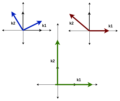
We can see there are three types of transformations shown above. Though they are not drawn to scale. First is the rotation, second is shear. The third one is the transformation found by multiplication of a matrix given below with the vectors of ij plane

Now, one thing to observe is in the first case both our i and j vectors change their direction, or let’s say the get deviated from their initial direction. In, the second case, the i vector (after transformation k1) remains in the same direction, though it’s value or magnitude as the unit vector may change. In the third case both the vector maintain their direction, but the magnitude changes, the i vector(now k1) becomes 2 times and the j vector (now k2) becomes 3 times.

The vectors of a system that does not change its direction(in simple words, avoiding the complications) after transformation are called the Eigenvectors. The eigenvectors though don’t change the directions but are scaled in terms of magnitude. For example, in the third case, i got scaled two times and j 3 times. These values by which the magnitude of eigenvectors gets scaled are called eigenvalues of the vectors. Now, one thing to note is it’s not only the i and j vectors, any vector belonging to the system which does not change the direction after transformation can be an eigenvector.

How to find the eigenvalue and vectors?

We saw for the eigenvectors after transformation just got scaled by a scalar value. We know transformation is matrix multiplication. So, it’s safe to say a scalar change in vector, when multiplied by a matrix. So, this is given by:

Av=(lambda)v

where A is the matrix, v is the eigenvector and lambda is the constant by which the vector gets scaled, so the eigenvalue.

So, we get the equation finally. Now the thing is, the equation will be 0 if v =0 but that’s too obvious, moreover we want v to be a non-zero vector.

We put (A-(lambda)I)=0 — — (1), so, we equate its determinant to be 0.

Actually there is another intuition behind this i.e, the determinant of a matrix, actually depicts the change in the area of the unit rectangle, that will take place if we transform a vector system using the matrix. For example, if we look at our third case, we scaled our unit vectors by 2 and 3 units. So, the current area of the unit rectangle is 6 which was initially 1. Now if we find the determinant of the transforming matrix,

We will find the determinant to be 6.

Returning to equation 1, we find the lambda values and find the eigenvectors accordingly.

How is PCA related?

For PCA, say we have two features X and Y. We first calculate the covariance matrix of X and Y.

Covariance is given by:

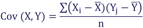
The covariance matrix is given by:

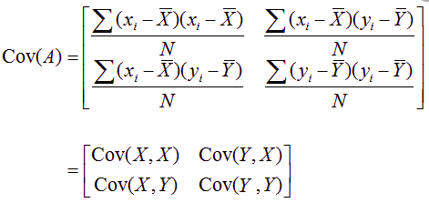
So, the covariance matrix is obtained from the features. Now we initialize any vector on the XY plane say, [-1 1].

We keep multiplying this vector again and again with the covariance matrix, the change or transformation of the vector slowly converges to a particular vector, which does not change. This gives eigenvector obtained for the plane.

For example, [-1 1] is our vector taken, and

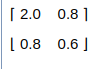
is the covariance matrix, obtained vector is [ x y] =[-2.5 -1.0]

y=-1.0

x=-2.5

So, -2.5i -1.0j is the vector obtained. The unit vector of the in the direction of this vector is the Eigenvector of the Principal Component 1.

Now,

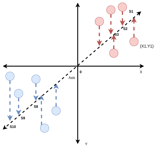
The sum of the square of distances S1, S2, S3………….S8, S9, S10 with 0 gives S.

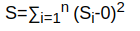
This S is called the variance in the direction of principal component 1.

Now, we consider another vector orthogonal to the eigenvector of component 1. It gives us the principal component 2.

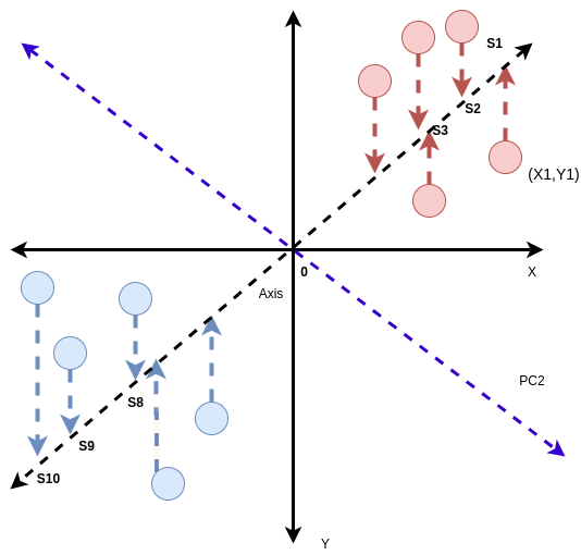
The violet line gives PC2. We find the S value for PC2 also as we did for PC1.

Now, say there N values in our distribution.

(Value of S for PC1 / N-1) gives the variation of PC1. Similarly, we find for PC2.

Now, if the variation of PC1 is 10 and PC2 is 2. Then,

PC1 accounts for 10/(10+2) x 100 =83% of the information represented.

For a 10 Dimensional Data these two components PC1 and PC2 may not represent most of the information and the formula gets modified as it will be having more components in the Denominator.

So, if we want to represent the X Y feature distribution using 1 principal component we will have 83% of the information represented.

Conclusion

In this article, we talked about the working of PCA.

Hope this helps.

---

Demystifying Principal Component Analysis was originally published in Towards AI — Multidisciplinary Science Journal on Medium, where people are continuing the conversation by highlighting and responding to this story.

Published via Towards AI