


Statistical Forecasting for Time Series Data Part 6: Forecasting Non-Stationary Time Series using…
Last Updated on January 6, 2023 by Editorial Team
Last Updated on December 26, 2020 by Editorial Team
Author(s): Yashveer Singh Sohi
Data Visualization
Statistical Forecasting for Time Series Data Part 6: Forecasting Non-Stationary Time Series using ARIMA
In this series of articles, the S&P 500 Market Index is analyzed using popular Statistical Model: SARIMA (Seasonal Autoregressive Integrated Moving Average), and GARCH (Generalized AutoRegressive Conditional Heteroskedasticity).
In the first part, the series was scrapped from the yfinance API in python. It was cleaned and used to derive the S&P 500 Returns (percent change in successive prices) and Volatility (magnitude of returns). In the second part, a number of time series exploration techniques were used to derive insights from the data about characteristics like trend, seasonality, stationarity, etc. With these insights, in the 3rd and 4th part the SARIMA and GARCH class of models were introduced. In the 5th part, the 2 models (SARIMA and GARCH) were combined to generate meaningful forecasts and derive accurate insights on future data. Links to all these parts are at the end of this article.
In this last part, the technique used to model Non-Stationary data using the SARIMA class of models are covered. The code used in this article is from Prices Models/ARMA Model for SPX Prices.ipynb notebook in this repository
Table of Contents
- Importing Data
- Train-Test Split
- Stationarity of S&P 500 Prices
- Converting S&P 500 Prices to a Stationary Series
- Modeling the Transformed Series
- Predicting S&P 500 Prices using ARMA Model
- Evaluating the Predictions
- Conclusions
- Links to other parts of this series
- References
Importing Data
Here we import the dataset that was scrapped and preprocessed in part 1 of this series. Refer part 1 to get the data ready, or download the data.csv file from this repository.
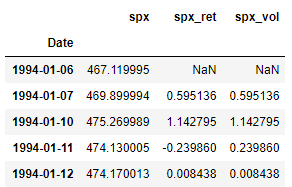
Since this is same code used in the previous parts of this series, the individual lines are not explained in detail here for brevity.
Train-Test Split
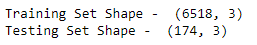
Like before, we now split the data into train test sets. Here all the observations on and from 2019–01–01 form the test set, and all the observations before that is the train set.
Stationarity of S&P 500 Prices
Before fitting any of the models from the ARIMA family, the stationarity of the input series should be checked. This is because in a stationary series the underlying process creating the data (the one ARIMA tries to model) will not change in the future. Hence the model will have a reasonable chance of success with stationary data.
To check whether a series is stationary or not, the following 3 ways are used:
- Check whether the data has no apparent trend (summary statistics do not change with time) using a line plot.
- Check the correlation of the plot with lagged versions of itself using the ACF and PACF plot.
- Check the results of the ADF (Augmented Dickey Fuller) Test. The Null Hypothesis states that the series is Non-Stationary. If the p-value returned is greater than all the critical levels, then the Null Hypothesis can not be rejected, and the series is not stationary. (A more in-depth description was provided in part2 of this series.)
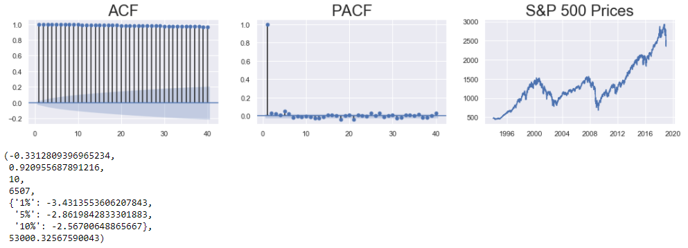
The correlation plots, and the line plots indicate a clear trend in the series. Additionally, the p-value of the ADF test is greater than all the critical levels, and hence the series is non-stationary.
Converting S&P 500 Prices to a Stationary Series
There are many techniques used to convert a non-stationary series to a stationary one. The following 2 are probably the most common ones:
- Differencing: Here the series is differenced with a lagged version of itself. The trend component of the series is usually removed in this transformation.
- Log Transform: Here the log of the series is calculated. The series is reduced in scale and the variations are damped in this transformation.
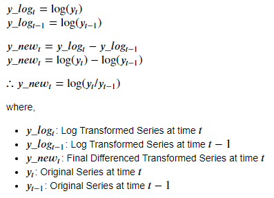
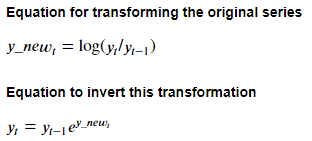
In this case, another common approach is used, which is to combine the above 2 approaches: Log-Differenced Transform. In this, first, the log of the series is calculated, and then the series is differenced with a lagged version of itself (here, lag is of 1 time period).
The mathematical formulation of this approach is:
The code to do this is as follows:
The stationarity of this new series can be checked in the same way as it was done for the original series. The train_df[“spx”] series is to be replaced by the train_df[“spx_log_diff”] series. The rest of the code can be the same as the one in the Stationarity of S&P 500 Prices section.
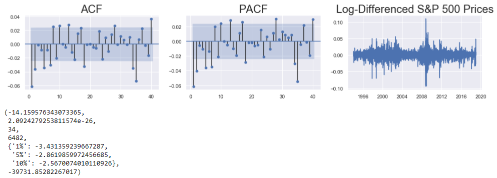
The correlation plots and the line plot indicate that the series is stationary (devoid of any obvious trend). The p-value of the ADF test gives further proof that the series is stationary.
Modeling The Transformed Series
Since the series is stationary, we can use the non-integrated variants of ARIMA models: AR, MA or ARMA. In this case, ARMA is chosen. The parameters of ARMA are denoted by ARMA(p, q):
- p: Controls the effect of past lags (estimated by counting the significant lags in PACF plot)
- q: Controls the effect of past residuals (estimated by counting the significant lags in ACF plot)
Looking at the ACF and PACF plots from the previous section, the initial estimates for these parameters can be: p=1 or p=2, and, q=1 or q=2 . Let’s consider the simplest of models: ARMA(1, 1).
The following code cell is used to build a ARMA(1, 1) model:
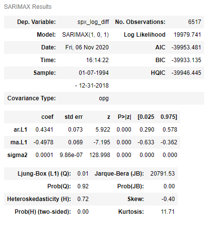
The SARIMAX() function is used to define the ARMA(1, 1) model by passing the transformed S&P 500 Prices series and the appropriate order as the arguments. The model is trained using the fit() method on the model definition. The summary table is displayed by using the summary() method on the fitted model.
The P<|Z| column of the summary table shows that all the coefficients of this model are significant. Next, this model is used to generate predictions for the transformed series, and then for the original prices series.
Predicting S&P 500 Prices using ARMA Model
For predicting the S&P 500 Prices, the ARMA(1, 1) model build previously will be used to forecast the values for the Transformed (Log-Differenced) S&P 500 Prices. Then the forecasted values (and confidence intervals) are reverse transformed to obtain the required values for the S&P 500 Prices.
Referring the transformation equation mentioned above, we can derive the reverse transformation using the following mathematical equations:
The code to derive the predictions for S&P 500 Prices is as follows:
- Firstly, a dataframe ( pred_df ) is defined that stores all the important series needed to derive the predictions for S&P 500 Prices.
- Next, the spx series and a lagged version of this series is stored in the dataframe. The lag is of 1 time period. These 2 series represent the y(t) and y(t-1) series in the formula shown above.
- Now, the model predictions are generated using the predict() method with the start and end dates specified on the fitted model. Also, the confidence intervals for these predictions are generated using the conf_int() method on the output of the get_forecast() function. These series represent the y_new(t) series and the confidence intervals for this series in the formula above.
- The exponent function is used on these predictions and their confidence intervals so as to generate the exp(y_new(t)) series from the formula above.
- Finally the lagged spx values ( y(t-1) ) and exp(y_new(t)) series generated previously are multiplied to get the desired predictions: y(t) .
Evaluating the Predictions
There are 2 ways in which the predictions generated previously are evaluated:
- Line plots of predictions along with the actual values
- Calculating the Root Mean Squared Error (RMSE) Metric
Code to generate the line plots and the RMSE metric is shown below:
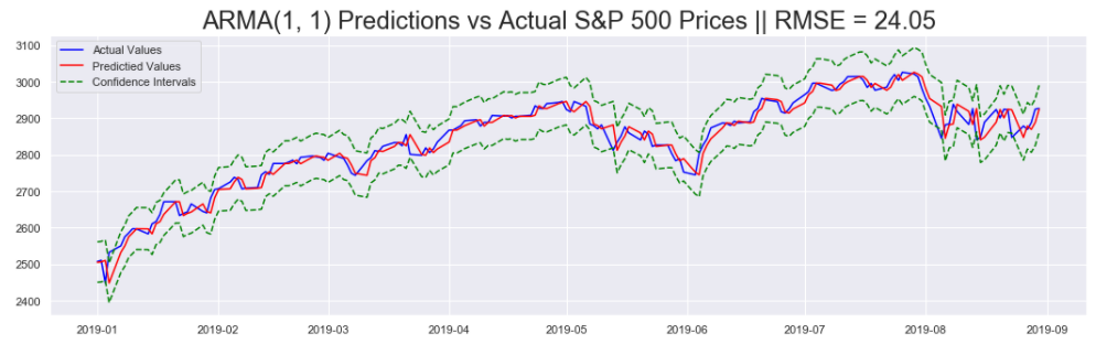
First the RMSE metric is calculated using the mean_squared_error() function from sklearn.metrics . Then the Predictions (In Blue) are plotted against the Actual S&P 500 Prices (In Red), along with the Confidence Intervals (In Green).
Conclusion
In this series of articles, the S&P 500 Market Index was analysed and modeled using Statistical Time Series Forecasting Models like SARIMA and GARCH. This series first covered ways to obtain such data, and, explore it for better understanding. Next, a couple of statistical models are introduced and applied on this data. Using these models we were able to predict future values and the margin of error associated with these predictions.
Links to other parts of this series
- Statistical Modeling of Time Series Data Part 1: Preprocessing
- Statistical Modeling of Time Series Data Part 2: Exploratory Data Analysis
- Statistical Modeling of Time Series Data Part 3: Forecasting Stationary Time Series using SARIMA
- Statistical Modeling of Time Series Data Part 4: Forecasting Volatility using GARCH
- Statistical Modeling of Time Series Data Part 5: ARMA+GARCH model for Time Series Forecasting.
- Statistical Modeling of Time Series Data Part 6: Forecasting Non — Stationary Time Series using ARMA
References
[1] 365DataScience Course on Time Series Analysis
[2] machinelearningmastery blogs on Time Series Analysis
[3] Wikipedia article on GARCH
[4] ritvikmath YouTube videos on the GARCH Model.
[5] Tamara Louie: Applying Statistical Modeling & Machine Learning to Perform Time-Series Forecasting
[6] Forecasting: Principles and Practice by Rob J Hyndman and George Athanasopoulos
[7] A Gentle Introduction to Handling a Non-Stationary Time Series in Python from Analytics Vidhya
Statistical Forecasting for Time Series Data Part 6: Forecasting Non-Stationary Time Series using… was originally published in Towards AI on Medium, where people are continuing the conversation by highlighting and responding to this story.
Published via Towards AI
Towards AI Academy
We Build Enterprise-Grade AI. We'll Teach You to Master It Too.
15 engineers. 100,000+ students. Towards AI Academy teaches what actually survives production.
Start free — no commitment:
→ 6-Day Agentic AI Engineering Email Guide — one practical lesson per day
→ Agents Architecture Cheatsheet — 3 years of architecture decisions in 6 pages
Our courses:
→ AI Engineering Certification — 90+ lessons from project selection to deployed product. The most comprehensive practical LLM course out there.
→ Agent Engineering Course — Hands on with production agent architectures, memory, routing, and eval frameworks — built from real enterprise engagements.
→ AI for Work — Understand, evaluate, and apply AI for complex work tasks.
Note: Article content contains the views of the contributing authors and not Towards AI.
Related posts


")
Recent Posts


")

