Finding Your Formula for Success: An Introduction to Linear Programming Through F1 Racing
Last Updated on June 28, 2023 by Editorial Team
Author(s): Monish kumar
Originally published on Towards AI.
Imagine yourself as an F1 team manager. Your task is simple yet intricate — design the perfect car for the upcoming Grand Prix. You have a variety of parts at your disposal, each contributing to the performance of your race car in distinct categories — Aero, Power, Handling, Lightweight, and Brakes.
You may think that attaching parts that boost power is an obvious solution. However, these same parts may decrease the braking ability, leading to high-speed turns becoming a high-risk challenge for your driver. Thus, your objective is to balance these conflicting elements to build the most competitive car on the grid.
This scenario mirrors the essence of decision-making in business, engineering, logistics, and various other fields, where resources must be optimally allocated under a set of constraints. This is where linear programming comes into play.
Linear Programming — A Formula1 of Decision Making
Linear programming is a mathematical approach used to achieve the best outcome in a mathematical model, such as maximizing profit, performance, or efficiency or minimizing cost, risk, or waste. Its applications span various fields, from logistics and supply chain management to production processes and portfolio optimization.
Now, back to our F1 scenario. With linear programming, you can figure out which parts to attach to each category to maximize your car’s overall performance based on your specific needs, whether it be more powerful or superior brakes. All of this while taking into account that only two parts can be attached per category.
Pit Stop — Laying out the Data
First, let’s break down the provided information.
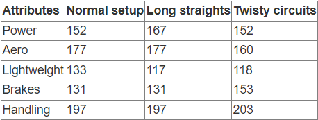
For our F1 car, we have five categories that we can modify:
- Power: Current level is 159, the chassis allows up to 81 additional points. Parts available are in the categories Power1 and Power2.
- Aero: Current level is 173, the chassis allows up to 122 additional points. Parts available are in the Aero category.
- Lightweight: Current level is 118, the chassis allows up to 81 additional points. Parts available are in the Lightweight category.
- Brakes: Current level is 144, the chassis allows up to 81 additional points. Parts available are in the Brakes category.
- Handling: Current level is 177, the chassis allows up to 121 additional points. Parts available are in the Handling1 and Handling2 categories.
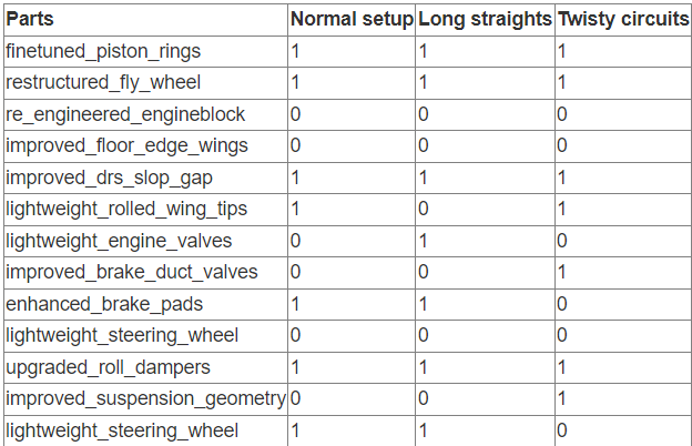
The selection of parts for each category is also provided, and each part has effects on the five attributes (either an absolute increase/decrease or a percentage increase). Remember, only two parts can be attached per category.
Race Strategy — Formulating the Problem
Formulating the problem in the language of linear programming involves defining our variables, objective functions, and constraints.
In this scenario, our variables are the choices of parts for each category. A binary variable can represent the choice of each part (1 if the part is chosen, 0 if not).
#variables
var finetuned_piston_rings binary;
var restructured_fly_wheel binary;
var re-engineered_engineblock binary;
Our objective function will likely be a weighted sum of the final attributes of the car. These weights represent our preference for each attribute. For example, if we valued power and aero more, we would assign them higher weights.
#Objective
maximize Z: 1*chassis_power + 1*chassis_aero + 1*chassis_lightweight + 1*chassis_brakes + 1*chassis_handling;
The constraints are the limitations on the number of parts we can use in each category (<= 2), the effect each part has on the attributes, and the maximum number of additional points the chassis allows.
#Constraints
subject to c_power1: finetuned_piston_rings + restructured_fly_wheel + re-engineered_engineblock = 2;
subject to c_aero: improved_floor_edge_wings + improved_drs_slop_gap = 1;
subject to c_lightweight: lightweight_rolled_wing_tips + lightweight_engine_valves = 1;
subject to c_brakes: improved_brake_duct_valves + enhanced_brake_pads = 1;
subject to c_handling: tyre_blanket + upgraded_roll_dampers + improved_suspension_geometry + lightweight_steering_wheel = 2;
subject to c_Power: finetuned_piston_rings*31 + restructured_fly_wheel*40 + re-engineered_engineblock*38 + improved_floor_edge_wings*0 + improved_drs_slop_gap*0 + lightweight_rolled_wing_tips*0 + lightweight_engine_valves*15 + improved_brake_duct_valves*0 + enhanced_brake_pads*0 + lightweight_steering_wheel*0 + upgraded_roll_dampers*0 + improved_suspension_geometry*0 + lightweight_steering_wheel*0 + 81 >= chassis_power;
Likewise, you have constraints for all 5 categories. In these constraints, the performance effect of each part is multiplied by the corresponding variable (i.e., the decision to use the part). If a part is not used, its variable is 0, and therefore it has no effect on the total. If it is used, the variable is 1, and the performance effect is added to the total. The total performance effect of the parts must be less than or equal to the maximum allowed by the chassis.
Into the Pits — The Linear Programming Model
Once the problem is formulated, it can be represented using a linear programming model. This model consists of an objective function that we want to maximize (or minimize) and a set of constraints that the solution must adhere to. The objective function will be a linear equation based on our variables — the parts we can attach — and the constraints will also be a series of linear equations or inequalities.
Once we have all these elements, we can input them into a linear programming solver such as Python’s GLPK, PuLP, SciPy, or AMPL libraries. Here I have used the GLPK solver, which is a basic and reliable linear solver. You can try out the solver for free at this link.
Green Lights — Finding the Optimal Solution
Now that we have our model, it’s time to solve it. This involves finding the values for our variables (the parts we will use) that will provide the highest value for our objective function (the overall performance) while adhering to our constraints. This solution represents the optimal way to attach the parts to our F1 car.
Remember, though, that different objectives may lead to different solutions. If we’re preparing for a race on a track with long straights, we may want to focus more on power and aerodynamics than handling.
#Objective
maximize Z: 1.5*chassis_power + 1.5*chassis_aero + 1*chassis_lightweight + 1*chassis_brakes + 1*chassis_handling;
Conversely, on a tight and twisty circuit, we might prioritize handling and brakes. This is akin to setting a different objective function.
#Objective
maximize Z: 1*chassis_power + 1*chassis_aero + 1*chassis_lightweight + 1.5*chassis_brakes + 1.5*chassis_handling;


This is the beauty of linear programming: it allows us to make informed, optimized decisions based on our specific needs and constraints.
Mapping the Track — Visualizing Linear ProgrammingU+1F3CE️
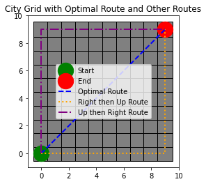
Imagine you are looking at a map of a city. Each city block is perfectly square, and your goal is to travel from one corner of the city to the opposite corner. You can only travel along the streets, not through the buildings. The most direct path, as the crow flies, is a straight diagonal line, but since you’re restricted to the grid of the streets, you’ll need to find an optimal route.
In our case, the ‘city’ is a multi-dimensional space of all the possible values of our variables (the different parts we can select), and the ‘corners’ of the city are our constraints (limitations on the number of parts per category and their effects on the car’s performance).

Linear programming works by ‘exploring’ this city, moving along the streets (testing different combinations of variables) to find the path that will get us to our goal (maximizing the sum of the car’s attributes) the fastest.
In the case of our F1 racing problem, the ‘city’ is a multi-dimensional space where each dimension represents a part selection, and the ‘corners’ are the constraints on part selection and the effects of parts on the car’s performance. The linear programming solver explores this city to find the combination of parts that will maximize the car’s performance.
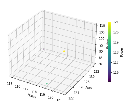
Given the provided data, we could visualize only a small fraction of the potential solutions in a 3D space. Let’s consider the Power, Aero, and Brakes parameters from three potential setups. We’ll do this with a single sample, although an actual implementation would likely involve a much larger range of possible setups.

When LP solver finds an optimal solution, it’s effectively finding the best point in this space according to your objective function (assuming it’s a maximization problem, it would be the point with the highest ‘Power’, ‘Aero’, and ‘Brakes’ value that still meets the constraints).
In conclusion, like a Grand Prix, solving linear problems can be a thrilling race. From formulating the problem to taking the checkered flag, each step brings us closer to our podium: optimal decision-making. As our F1 scenario illustrates, linear programming is a versatile tool that can help us steer toward success, no matter the challenge.
Join thousands of data leaders on the AI newsletter. Join over 80,000 subscribers and keep up to date with the latest developments in AI. From research to projects and ideas. If you are building an AI startup, an AI-related product, or a service, we invite you to consider becoming a sponsor.
Published via Towards AI
Towards AI Academy
We Build Enterprise-Grade AI. We'll Teach You to Master It Too.
15 engineers. 100,000+ students. Towards AI Academy teaches what actually survives production.
Start free — no commitment:
→ 6-Day Agentic AI Engineering Email Guide — one practical lesson per day
→ Agents Architecture Cheatsheet — 3 years of architecture decisions in 6 pages
Our courses:
→ AI Engineering Certification — 90+ lessons from project selection to deployed product. The most comprehensive practical LLM course out there.
→ Agent Engineering Course — Hands on with production agent architectures, memory, routing, and eval frameworks — built from real enterprise engagements.
→ AI for Work — Understand, evaluate, and apply AI for complex work tasks.
Note: Article content contains the views of the contributing authors and not Towards AI.


