Logo:
Logo:  Areas Served:
The Infamous Attention Mechanism in the Transformer Architecture
Last Updated on April 22, 2024 by Editorial Team
Author(s): Arion Das
Originally published on Towards AI.
THE WHY & WHEN?
It all started with a problem. How do you play around with sequential data?! People had the architecture to work with regression and classification problems, but sequential data was very different.
So, a new neural network architecture was introduced that had the concept of memory to enable working with sequential data. RNNs (LSTMs & GRUs).

RNNs & LSTMs did help provide the output to a sequential input, but then came another challenge. What if the output is also a sequence ?! Unfortunately, the architecture faltered. This is where the concept of sequence-to-sequence neural networks came into the picture.
THE SUTSKEVER ARCHITECTURE

The simplest strategy for general sequence learning was to map the input sequence to a fixed-sized vector using one RNN, and then to map the vector to the target sequence using another RNN. The statistical machine translation paper by Kyunghun Cho did the same.

However, this didn’t prove feasible, as it would be difficult to train the RNNs due to long-term dependencies. An obvious alternative was LSTMs.
The goal of the LSTM was to estimate the conditional probability p(y1,…,yT′|x1,…,xT), where (x1,…,xT) is an input sequence and (y1,…,yT′) is its corresponding output sequence.
Note how their lengths, T & T', may differ.
THE ENCODER-DECODER WORKFLOW
This is done by first obtaining the fixed-dimensional representation, v (the context vector), of the input sequence (x1,…,xT), given by the last hidden state of the LSTM (encoder). It then computes the probability of (y1,…,yT′) with a standard LSTM-LM formulation whose initial hidden state is set to the context vector (decoder).

HOW SUTSKEVER’s MODEL DIFFERED
- Two different LSTMs were used for the input & output sequences. This helped increase the model parameters (at negligible cost) and helped train the LSTM on multiple language pairs simultaneously.
- Deep LSTMs outperformed shallow LSTMs as they could recognize hierarchical patterns. So, a LSTM with 4 layers was chosen.
- The input sequence was reversed. This reduced the distance between a word (in the first half) of the input sequence & it’s corresponding output word. This resulted in less computational loss during backpropagation. But this helped with languages that have their context in the first few words and whose output sequence is of a small length.
It turns out, the model did work well, achieving a BLEU score of 34.18 compared to the baseline score of 33.30.
ISSUES WITH THE SEQ-2-SEQ MODEL
- The context vector produced by the encoder was of fixed size.
- This made it incapable of remembering long term dependencies.
- It used to forget the first part once the whole input was processed.
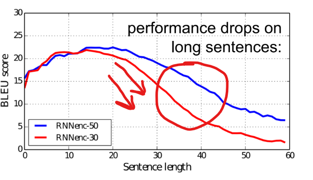
- Long sentences deviate from the required context.
THE ATTENTION MECHANISM (Self Attention)
Upon closer inspection, you’ll realize something is being done needlessly.
Why are we using the entire input sequence every time for the next word prediction?!!
INTUITION
Imagine reading some text. At any instant, our eyes focus on two to three words at maximum. This is when our attention is being given to that particular phrase. Similarly, for the next word prediction, we don’t need the entire input sequence every time; we just need some closely related phrases from the input sequence (attentive ones!!). So, in predicting a certain word, we are being attentive to certain phrases.
Clearly, we need some highlighted parts of the input text that will be responsible for the next token in the sequence. Now, how do we recognize which parts of the input sequence are required for the next token prediction?
THE MATH
Inputs
- ‘n’ query vectors : q1, q2, q3,…, qn
- ‘m’ key vectors : k1, k2, k3,…, km
- ‘m’ value vectors : v1, v2, v3,… vm
Output
‘n’ output vectors : o1, o2, o3,… on
The output vectors are computed using the relations between the corresponding query vector and each key vector as coefficients.
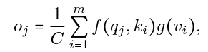
Here, f(qj, ki) is a commonly used similarity function which denotes the relation between qj & ki. ‘C’ is a normalization factor, & ‘g’ performs a linear transformation.
When expressed in matrix form,

Q (dXn) is a matrix containing the query vectors, K (dXm) the key vectors, & V (pXm) the value vectors. O (qXn) contains the output vectors. Softmax normalizes the input matrix.

Note how the transpose of K makes it compatible for matrix multiplication with Q. Also, the number of output vectors is equal to the number of query vectors.
I won’t get into much detail about how we are preparing the embeddings for our query, key, & value matrices (I’ll do that in the transformer blog), but here is a small snippet that shows the sequence of actions to be taken.
FOR HACKERS
import torch
import torch.nn as nn

class Attention(nn.Module):
 def __init__(self, input_dim):
 super(SelfAttention, self).__init__()
 self.input_dim = input_dim
 self.query = nn.Linear(input_dim, input_dim)
 self.key = nn.Linear(input_dim, input_dim)
 self.value = nn.Linear(input_dim, input_dim)
 self.softmax = nn.Softmax(dim=2)

 def forward(self, x):
 queries = self.query(x)
 keys = self.key(x)
 values = self.value(x)
 scores = torch.bmm(queries, keys.transpose(1, 2)) / (self.input_dim ** 0.5)
 attention = self.softmax(scores)
 weighted = torch.bmm(attention, values)
 return weighted
The query, key, and value vectors are learned through linear transformations of the input sequence.
The attention scores are then calculated as the dot product of the queries and keys, and the attention is applied by multiplying the values by the attention scores. A weighted representation of the input sequence is obtained as a result.
BAHDANAU ATTENTION (Additive Attention)
|| paper ||
Prior machine translation techniques had the same issue. They had to compress all the information of a source sentence into a fixed-length vector. This resulted in rapid deterioration of performance in case of longer sentences.
Their novelty was that they did not attempt to encode the entire input sequence. Instead, they encoded the input sequence into a sequence of vectors and chose a subset of these vectors while decoding.
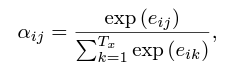
Alignment Score (alpha)
This is the metric which determines the extent of alignment / similarity of the i-th word across the available input sequence vectors.
Now, on what factors does this score depend upon?
Clearly, it depends on the hidden encoder layer. But here’s the catch. It also depends on what has already been translated i.e. the previous hidden decoder layer.
So, now that we have the two inputs, we can pass them through a feed forward neural network, which will provide us with an approximate mathematical function.

Now that we have all the alignment scores and the previous hidden encoder layer, we can use them to calculate c-i, the context vector (for the i-th word prediction), on which the prediction of the next token will depend.
Clearly, in this architecture, the decoder decides which parts of the source sentence to pay attention to. So, the encoder doesn’t have to encode all the information in the source sentence to a fixed length vector. This new approach helps spread the information throughout the sequence of annotations, which can then be selectively retrieved by the decoder.

FOR HACKERS
class Attention(nn.Module):
 def __init__(self, enc_hid_dim, dec_hid_dim):
 super().__init__()

 self.attn = nn.Linear((enc_hid_dim * 2) + dec_hid_dim, dec_hid_dim)
 self.v = nn.Linear(dec_hid_dim, 1, bias = False)

 def forward(self, hidden, encoder_outputs):

 batch_size = encoder_outputs.shape[1]
 src_len = encoder_outputs.shape[0]

 #repeating decoder hidden state src_len times
 hidden = hidden.unsqueeze(1).repeat(1, src_len, 1)

 encoder_outputs = encoder_outputs.permute(1, 0, 2)

 energy = torch.tanh(self.attn(torch.cat((hidden, encoder_outputs), dim = 2)))

 #energy = [batch size, src len, dec hid dim]

 attention = self.v(energy).squeeze(2)

 #attention= [batch size, src len]

 return F.softmax(attention, dim=1)
Code courtesy of Maab Nimir.
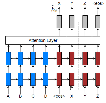
LUONG ATTENTION (Multiplicative Attention)
|| paper ||
Their architecture is pretty much similar to Bahdanau’s but for a couple of differences:
- Instead of the previous hidden decoder state, the current decoder state is used.
- Instead of a feed forward neural network, dot product between the hidden encoder & decoder layers works as the mathematical function here.
The ‘energy’ term produced from the dot product is normalized using softmax which gives us the alpha value (alignment score).
Advantages
- The feed forward neural net meant a pretty complex mathematical formula using multiple parameters (to replicate the patterns), resulting in very slow computation. Dot products take much less time.
- Using the current hidden decoder state helped in using more updated information, helping the output get adjusted more dynamically.
Note that here the context vector calculated using the alignment scores is concatenated with the output of each state rather than with the input (in Bahdanau).
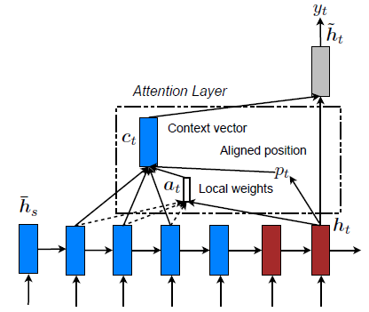
The above image shows the current hidden decoder state being provided as an input to inform about past alignment decisions.
FOR HACKERS
class DotProductAttention(nn.Module):
 def __init__(self, hidden_dim):
 super(DotProductAttention, self).__init__()

 def forward(self, query: Tensor, value: Tensor) -> Tuple[Tensor, Tensor]:
 batch_size, hidden_dim, input_size = query.size(0), query.size(2), value.size(1)

 score = torch.bmm(query, value.transpose(1, 2))
 attn = F.softmax(score.view(-1, input_size), dim=1).view(batch_size, -1, input_size)
 context = torch.bmm(attn, value)

 return context, attn
Code courtesy of Soohwan Kim.
A quick recap on self-attention:
- We generate contextual embeddings from the source sentence.
- These are then broken into 3 matrices: query, key & value
- Now, we use the self-attention formula to generate a set of output vectors, which are then used to provide a response.
PROBLEM WITH SELF ATTENTION
Consider the sentence:
“Hang them not let them go.”
Meaning 1: Don’t hang the people, let them go.
Meaning 2: Hang the people, don’t let them go.
Clearly, the given sentence might have either of the perspectives. Unfortunately, self attention is capable of capturing any one of these perspectives. To overcome this problem, we use the concept of multi-head attention.
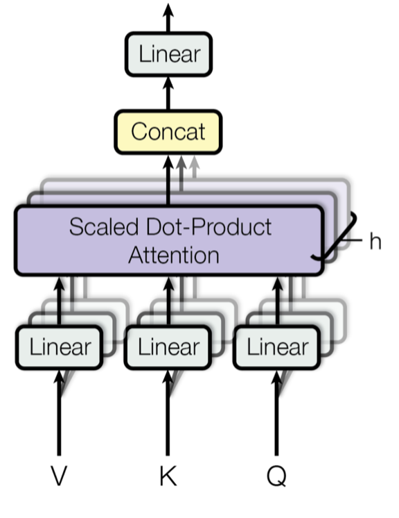
MULTI-HEAD ATTENTION
Quite simply, as it’s name suggests, we use multiple self attention blocks together.
Essentially, we run several self attention blocks which run in parallel. The independent attention outputs are then concatenated and linearly transformed into the required dimension. It allows us to cater to both longer term and shorter-term dependencies, helping us capture the exact perspective being used.
MultiHead(Q,K,V) = [attn(1), attn(2),…, attn(h)] Wo
here, head(i) = Attention(QW(i)(Q), KW(i)(K), VW(i)(V))
Scaled dot-product is the most common here, & W represents all learnable parameters.
FOR HACKERS
class MultiheadAttention(nn.Module):

 def __init__(self, input_dim, embed_dim, num_heads):
 super().__init__()
 assert embed_dim % num_heads == 0, "Embedding dimension must be 0 modulo number of heads."

 self.embed_dim = embed_dim
 self.num_heads = num_heads
 self.head_dim = embed_dim // num_heads

 # Stacking all weight matrices 1...h together for efficiency
 self.qkv_proj = nn.Linear(input_dim, 3*embed_dim)
 self.o_proj = nn.Linear(embed_dim, embed_dim)


 def forward(self, x, mask=None, return_attention=False):
 batch_size, seq_length, _ = x.size()
 if mask is not None:
 mask = expand_mask(mask)
 qkv = self.qkv_proj(x)

 # Separating Q, K, V from linear output
 qkv = qkv.reshape(batch_size, seq_length, self.num_heads, 3*self.head_dim)
 qkv = qkv.permute(0, 2, 1, 3) # [Batch, Head, SeqLen, Dims]
 q, k, v = qkv.chunk(3, dim=-1)

 # Determining output values
 values, attention = scaled_dot_product(q, k, v, mask=mask)
 values = values.permute(0, 2, 1, 3) # [Batch, SeqLen, Head, Dims]
 values = values.reshape(batch_size, seq_length, self.embed_dim)
 o = self.o_proj(values)

 return o, attention
Code courtesy of Analytics Vidhya.
That’s pretty much the underlying math behind various types of attention mechanisms. In the next blog, I’ll discuss the transformer architecture and how it’s being applied in various domains to produce efficient architectures.
Let’s connect and build a project together: 🐈⬛

Join thousands of data leaders on the AI newsletter. Join over 80,000 subscribers and keep up to date with the latest developments in AI. From research to projects and ideas. If you are building an AI startup, an AI-related product, or a service, we invite you to consider becoming a sponsor.
Published via Towards AI
Related posts
Popular posts

 for 2021")


Updates

Recent Posts