


 using Pyspark")
Exploratory Data Analysis (EDA) using Pyspark
Last Updated on July 24, 2023 by Editorial Team
Author(s): Vivek Chaudhary
Originally published on Towards AI.
Data Analytics, Python
The objective of this article is to perform analysis on the dataset and answer some questions to get the insight of data. We will learn how to connect to Oracle DB and create a Pyspark DataFrame and perform different operations to understand the various aspect of the dataset.
Exploratory Data Analysis or (EDA) is an understanding of the data sets by summarizing their main characteristics.
As this is my first Blog on EDA, so I have tried to keep the content simple just to make sure I resonate with my readers. So without wasting further a minute lets get started with the analysis.
1. Pyspark connection and Application creation
import pyspark
from pyspark.sql import SparkSession
spark= SparkSession.builder.appName(‘Data_Analysis’).getOrCreate()
2. Pyspark DB connection and Import Datasets
#Import Sales Data
sales_df = spark.read.format(“jdbc”).option(“url”, “jdbc:oracle:thin:sh/sh@//localhost:1521/orcl”).option(“dbtable”, “sales”).option(“user”, “sh”).option(“password”, “sh”).option(“driver”, “oracle.jdbc.driver.OracleDriver”).load()#Import Customer Datacust_df = spark.read.format(“jdbc”).option(“url”, “jdbc:oracle:thin:sh/sh@//localhost:1521/orcl”).option(“dbtable”, “customers”).option(“user”, “sh”).option(“password”, “sh”).option(“driver”, “oracle.jdbc.driver.OracleDriver”).load()#Import Products dataprod_df = spark.read.format(“jdbc”).option(“url”, “jdbc:oracle:thin:sh/sh@//localhost:1521/orcl”).option(“dbtable”, “products”).option(“user”, “sh”).option(“password”, “sh”).option(“driver”, “oracle.jdbc.driver.OracleDriver”).load()#Import Channels Datachan_df = spark.read.format(“jdbc”).option(“url”, “jdbc:oracle:thin:sh/sh@//localhost:1521/orcl”).option(“dbtable”, “channels”).option(“user”, “sh”).option(“password”, “sh”).option(“driver”, “oracle.jdbc.driver.OracleDriver”).load()#Import Country datacountry_df = spark.read.format(“jdbc”).option(“url”, “jdbc:oracle:thin:sh/sh@//localhost:1521/orcl”).option(“dbtable”, “countries”).option(“user”, “sh”).option(“password”, “sh”).option(“driver”, “oracle.jdbc.driver.OracleDriver”).load()
ojdbc6 is required for Oracle DB connection
3. Display the data
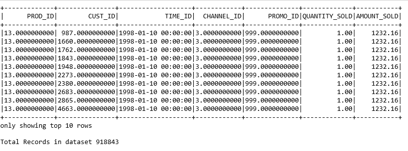
#sales data
sales_df.show(10)
print('Total Records in dataset',sales_df.count())
#customer data
cust_df.show(5)
print(‘Total Records in dataset’,cust_df.count())

#product data
prod_df.show(5)
print(‘Total Records in dataset’,prod_df.count())
#channels data
chan_df.show()
print(‘Total Records in dataset’,chan_df.count())

#Country data
country_df.show(5)
print(‘Total Records in dataset’,country_df.count())

4. Display schema and columns of DataFrame
#dataframe schema
sales_df.printSchema()

#display list of columns
sales_df.columns

5. Select and filter condition on DataFrame
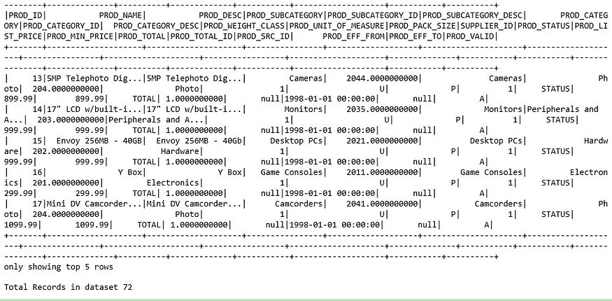
#select some columns from product dataframe
prod_df.select(‘PROD_ID’,
 ‘PROD_NAME’,
 ‘PROD_DESC’,’PROD_STATUS’,
 ‘PROD_LIST_PRICE’,
 ‘PROD_MIN_PRICE’,’PROD_EFF_FROM’,
 ‘PROD_EFF_TO’,
 ‘PROD_VALID’).show(7)

#filter condition with selective columns
country_df.select(‘COUNTRY_ID’,
 ‘COUNTRY_ISO_CODE’,
 ‘COUNTRY_NAME’,).filter(country_df.COUNTRY_NAME==’India’).show()
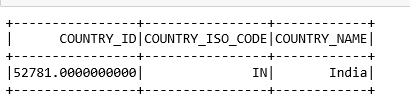
Typecast Column_ID to convert Decimal data to Integer data.
from pyspark.sql.types import IntegerType
country_df.select(country_df[‘COUNTRY_ID’].cast(IntegerType()).alias(‘COUNTRY_ID’),
 ‘COUNTRY_ISO_CODE’,
 ‘COUNTRY_NAME’,).filter(country_df.COUNTRY_NAME==’India’).show()

6. GroupBy and Aggregation
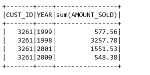
Let's find out how a customer spend in a year and over the span of 4 years from 1998–2002 find out customer spending in an individual year.
from pyspark.sql.functions import dayofyear,year
from pyspark.sql.functions import round, colsale_sum_df=sales_df.select(‘CUST_ID’,’TIME_ID’,’AMOUNT_SOLD’)cust_wise_df=sale_sum_df.groupBy(round(‘CUST_ID’,0).alias(‘CUST_ID’), year(sale_sum_df[‘TIME_ID’]).alias(‘YEAR’)).sum(‘AMOUNT_SOLD’)cust_wise_df.show(10)

7. Data Sorting
#Sort the records on basis of
cust_wise_df.orderBy(cust_wise_df.CUST_ID).show(15)

Lets check Year wise Customer spending.
cust_wise_df.filter(cust_wise_df.CUST_ID==3261).show()
8. Number of Customer visits over the time
sale_sum_df.groupBy(sale_sum_df[‘CUST_ID’].cast(IntegerType()).alias(‘CUST_ID’)).count().show(10)

9. Total Sale of a Product over the span of 4 years
s_df=sales_df.select(round(‘PROD_ID’,0).alias(‘PROD_ID’),year(sale_sum_df[‘TIME_ID’]).alias(‘YEAR’),’AMOUNT_SOLD’)
#withColumnRenamed changes column name
s_df=s_df.withColumnRenamed(‘PROD_ID’,’PROD_ID_S’)p_df=prod_df.select(‘PROD_ID’,’PROD_NAME’)
p_df=p_df.withColumnRenamed(‘PROD_ID’,’PROD_ID_P’)#join the above two dataframes created
prod_sales_df=s_df.join(p_df,p_df.PROD_ID_P==s_df.PROD_ID_S,how='inner')#perform groupby and aggregation to sum the sales amount productwise
prod_sales=prod_sales_df.groupBy('PROD_ID_S','PROD_NAME').sum('AMOUNT_SOLD')
prod_sales=prod_sales.select(col('PROD_ID_S').alias('PROD_ID'),'PROD_NAME',col('sum(AMOUNT_SOLD)').alias('TOTAL_SALES'))
prod_sales.show(10)

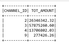
10. Channel wise Total Sales
#find out which channel contributed most to the salesc_df=chan_df.select(col(‘CHANNEL_ID’).alias(‘CHANNEL_ID_C’),col(‘CHANNEL_DESC’).alias(‘CHANNEL_NAME’))sa_df=sales_df.select(col(‘CHANNEL_ID’).alias(‘CHANNEL_ID_S’),’AMOUNT_SOLD’)chan_sales_df=sa_df.join(c_df,c_df.CHANNEL_ID_C==sa_df.CHANNEL_ID_S,how=’inner’)
chan_sale=chan_sales_df.groupBy(round(‘CHANNEL_ID_C’,0).alias(‘CHANNEL_ID’)).sum(‘AMOUNT_SOLD’)chan_top_sales=chan_sale.withColumnRenamed(‘sum(AMOUNT_SOLD)’,’TOT_AMOUNT’)chan_top_sales.orderBy(‘CHANNEL_ID’).show()
Summary
· Pyspark DB connectivity
· Data display using show()
· Schema and columns of Dataframe
· Apply select and filter condition on DFs
· GroupBy and Aggregation
· Column renames
· Some Data Insights
Hurray, here we completed Exploratory Data Analysis using Pyspark and tried to make data look sensible. In upcoming articles on Data Analysis, I will share some more Pyspark functionalities.
Join thousands of data leaders on the AI newsletter. Join over 80,000 subscribers and keep up to date with the latest developments in AI. From research to projects and ideas. If you are building an AI startup, an AI-related product, or a service, we invite you to consider becoming a sponsor.
Published via Towards AI
Towards AI Academy
We Build Enterprise-Grade AI. We'll Teach You to Master It Too.
15 engineers. 100,000+ students. Towards AI Academy teaches what actually survives production.
Start free — no commitment:
→ 6-Day Agentic AI Engineering Email Guide — one practical lesson per day
→ Agents Architecture Cheatsheet — 3 years of architecture decisions in 6 pages
Our courses:
→ AI Engineering Certification — 90+ lessons from project selection to deployed product. The most comprehensive practical LLM course out there.
→ Agent Engineering Course — Hands on with production agent architectures, memory, routing, and eval frameworks — built from real enterprise engagements.
→ AI for Work — Understand, evaluate, and apply AI for complex work tasks.
Note: Article content contains the views of the contributing authors and not Towards AI.
Related posts
Recent Posts


")


