(Part I) Fostering Criminal Justice with Data Science

Author(s): Vincent Liu

Originally published on Towards AI.

A Data-driven Analysis of the Uniform Crime Report 2021 DC Arrest Data

As a crime researcher, I am always intrigued by the questions of how many crimes were committed in a year and, out of these crimes, how many arrests were made by officers. I explicitly mentioned arrests here because these two concepts are distinct in the sense that not all crimes result in an arrest. Most cases simply do not amount to the level of seriousness needed to validate an arrest, for which should our attention is on behavioral biases of law enforcement agents (racial discrimination in policing), the arrest usually is often a better metric.

In this post, I will be using data from the Uniform Crime Reporting (UCR) system to tell a story about who was arrested in DC — the nation’s capital and political center — in 2021, the passing year. I especially care about these three questions:

• Which racial, sex, or age groups were arrested the heaviest by Metropolitan Police Department officers?
• How were those arrests broken down by offense type and weapon use
• Was a certain racial or socioeconomic group more likely to be arrested for some types of offenses?

While answering these questions, I will also show what I have been advocating for: using data science as a tool to understand the domain knowledge. I come from a social science background, and my interest in social science precedes my interest in data science. Accordingly, I believe that the importance of data science is that it provides tools for research scientists, policymakers, and companies. A lot of people in the data science field care more about the data algorithm than the data itself. I think they are of equal significance.

What is UCR, and Why UCR Crime Data?

I chose UCR as my source of data for a reason. When I was undergraduate sociology of law, criminology, and deviance student at the University of Minnesota Twin Cities, Uniform Crime Report (UCR) data was the common “guest” in many of my major courses that a lot of us called it “the bible of crime research”. This is not to say UCR is the best source but that it is the most authoritative one. Its authoritativeness reflects two points: it comes from a highly credible source (collected by the FBI), and it is very comprehensive (contains a myriad of information about crimes). No matter whether the researcher cares about the specific crime or arrest numbers in their living state or crime trends over the past decade, UCR is their go-to dataset.

UCR does not refer to a single data, but a data reporting system used by the FBI and is comprised of over five distinct databases. Some of the more well-known ones include the National Incident-Based Reporting System (NIBRS), the Hate Crime Statistics, the Law Enforcement Officers Killed and Assaulted data, and the most recent National Use-of-Force Data Collection. Data in the UCR system comes from over 18,000+ academic institutions and law enforcement agencies of different levels who reported crime information voluntarily.

Now, let’s take a look at our data.

Getting the Data and Setting up: Rising the Heat

The 2021 DC arrest data is grasped from the National Incident-Based Reporting System (NIBRS) database, which can be accessed on the FBI’s Crime Data Explorer portal. To download the data, go to the “Crime Incident-Based Data by State” section, select “DC” and “2021” in dropdowns, and press “download”. This will give you a set of related datasets and their codebooks in a compressed form, and the arrest data is among them!

Before moving to real data science tasks, it’s always a good habit to load libraries first.

library(dplyr) # for easy data cleaning and wrangling
library(forcats) # dealing with factor variables
library(stringr) # string manipulations
library(ggplot2) # data visualizations
library(GGally) # an extension of the ggplot2 library
library(lubridate) # dealing with dates and times
library(readr) # reading data
library(kableExtra) # beautiful formatting of tables

We will need two datasets: the arrest data and the arrest_by_weapon data. The former records the time and nature of arrests, while the latter complements the former by adding information about the use of weapons by the offenders. To connect them, we do a left join, which retains all rows in data x during joining (syntax: left_join(x,y, by = “”)). I named the joined dataset dc21_arrests_weapon.

dc21_arrests <- read_csv("data/DC2021_NIBRS_ARRESTEE.csv")
dc21_weapon <- read_csv("data/DC2021_NIBRS_ARRESTEE_WEAPON.csv")dc21_arrests_weapon <- dc21_arrests %>%
 left_join(
 dc21_weapon, 
 by = "arrestee_id")

Note that some rows in dc21_weapon appear more than one-time for which doing a join, regardless of the join type, will always include the repetitive rows in the result dataset. This can be easily tested with the method below (no warning message means the test passed, i.e. both conditions rendered the same output).

testthat::expect_equal(dc21_arrests %>% count(arrestee_id) %>% nrow(),
 dc21_weapon %>% count(arrestee_id) %>% nrow())

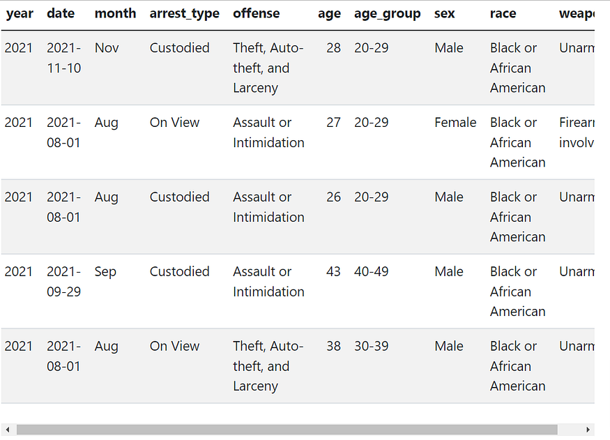
Let’s look at what’s in the data. We do so by inspecting the first five rows and glimpsing variable types.

dc21_arrests_weapon %>%
 head(5) %>% 
 kbl(format="html") %>%
 kable_styling(bootstrap_options = c("striped", 
 "hover", 
 "condensed"))

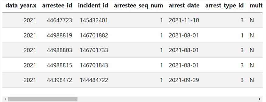
There are quite a few ways to check variable types. Many people love to use glimpse() since it’s well integrated with the tidyverse system. Here, I used base R’s str() method because I really like its layout. Both methods did very similar things, so there isn’t a trade-off here. Just use whichever you prefer.

str(dc21_arrests_weapon)
#dc21_arrests_weapon %>% glimpse() # alternative way

Here we see the data has 4,508 rows and 21 columns. The former suggests that in the year 2021, there were a total of 4,508 arrests in DC, whereas, the latter tells us that 21 variables are included in this data. Most of them are numeric, some are strings, and there are a few that are booleans (logi) and the data type. Examining variable types helps us understand our data better and makes our data cleaning easier.

Cleaning and Wrangling the Data: Making Hands Dirty

Let’s move to the data-cleaning stage. I think one reason why I really like data cleaning is that it is so logical and systematic. When we find unused variables, we drop them, and if something is not right, we manipulate and manipulate them with as many steps as needed and as few steps as possible. We also clean data one step at a time, and after a step, we look back to see if we did it right. In fact, we need to constantly look back and make changes to our previous codes to ensure we do not deviate from the right track. The mindset will also help us, (rising or experienced) data scientists be more familiar with and develop a stronger understanding of our data.

For me, data cleaning actually made me get into the field of data science. When I learned R programming in my undergraduate as a statistics major (I pursued two majors), there was no class about dplyr or ggplot2 and I learned how to clean data by myself in two weeks while working on a data science project. It wasn’t easy at the beginning because the tidyverse syntax is so different from base R, however, the more I used it, the more I found myself addicted to it. As I said, I came from a research background, so the problem-driven mindset inside the tidyverse framework is so natural and intuitive to me, which made me love doing data cleaning almost instantly.

Selecting Variables of Interest

Going back to our data, we need to do a few things before the most exciting part — explorative data analysis. We need to remove unnecessary variables so that our data only captures the main points of our analysis. This is especially important if our data has a few hundred columns, which could be common in the public and nonprofit sectors. For the one we are analyzing, there are 21 variables, which is a moderate number, so data selection is not necessary, but it never hurts to do so. We have to be cautious, though, to ensure we don’t filter out variables that we actually need. To do that, it’s often necessary to look for a codebook or an online code documentation page to make sure we are not being subjective about our variable interpretations. A codebook of the NIBRS dataset can be found on the same page we download our data or accessed here.

Out of these 21 variables, we found out arrest_id, incident_id, arrestee_sql_num are all used to identify arrests/arrestees, and variables age_id, age_num, under_18_disposition_code, age_range_low_num, age_range_high_num all represent arrestees’ age (we have the variable variation here because juveniles go through a different prosecution system and are often coded divergently from adults to protect their privacy). Moreover, there are a few variables that are out of the bond of our topic and thus, filtered out.

It turns out that we only kept 8 variables. I have also renamed these variables so that their names are more reflective of what they mean.

dc21 <- dc21_arrests_weapon %>%
 select(data_year.x, arrest_date, arrest_type_id, offense_code, 
 age_id, sex_code, race_id, weapon_id) %>%
 rename(year = data_year.x, 
 date = arrest_date,
 arrest_type = arrest_type_id,
 offense = offense_code, 
 age = age_id,
 sex = sex_code,
 race = race_id,
 weapon = weapon_id)

Variable Manipulation

Now, noticed that race, arrest_type, and weapon are labeled numerically, which is a common practice in data entry. However, it’s hard to know what each number means without referencing the codebook. Therefore, let’s do some re-coding, starting from the variable race.

Through some simple manipulations, we found race has 6 categories with categories 30, 40, and 50 having under 20 arrest cases. Because their numbers are so small compared to other racial groups, we can combine them together. Category 98 represents arrestees whose racial information is unknown, either because the officer forgot to write it down (it happens!) or for some other reason and is dropped out.

I am using functions from the forcats package to simplify the task

dc21 %>%
 count(race) # see what racial groups we have

dc21 <- dc21 %>%
 filter(!race == "98") %>%
 mutate(race = factor(race)) %>%
 mutate(race = fct_collapse(race,
 White = "10",
 `Black or African American` = "20",
 `Asian` = "40",
 `American Indian or Pacific Islander` = c("30","50")
 )) %>%
 mutate(race = fct_relevel(race, # relevel
 "Black or African American",
 after = 1)) %>%
 mutate(race = fct_relevel(race, # relevel
 "Asian",
 after = 2))

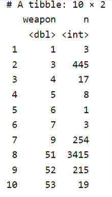
Repeating the process to variables weapon and sex. For sex, all we need is renaming factors.

dc21 %>%
 count(weapon)

dc21 <- dc21 %>%
 mutate(weapon = factor(weapon)) %>%
 mutate(weapon = fct_collapse(weapon,
 Unarmed = "51",
 `Firearm-involved` = c("1", "3", "4", "5", "6", "7", "9"),
 `Weapon with a blade` = c("52", "53")
 )) %>%
 mutate(weapon = fct_relevel(weapon, 
 "Firearm-involved",
 after = 1))

The fct_recode function offers an easy solution to recode factor levels. Alternatively, you can use base R’s recode function to do the same.

dc21$sex = fct_recode(dc21$sex, Male = "M", Female = "F")

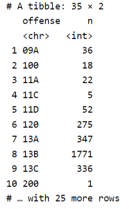
For offense, we need to have some extra considerations. Noticed that most offenses categories are made up of two components: a two-digit number and a letter. These two components respectively represent the first group and second group of offenses. For instance, 13 represents assaults, and the A, B, and C that comes after 13 specify the type and degree of assaults so that 13A represents aggravated assaults while 13B represents simple assaults. This classification approach has important legal and policy meanings. We can also utilize this classification approach to reduce our workloads.

dc21 %>%
 count(offense)

dc21 <- dc21 %>%
 mutate(offense = factor(offense)) %>%
 mutate(offense = fct_collapse(offense,
 `Murder and Nonnegligent Manslaughter` = "09A",
 `Aggravated Assault` = "13A",
 `Assault or Intimidation` = c("13B", "13C"),
 `Sexual Assault or Rape` = c("11A", "11C", "11D"),
 `Robbery` = c("120"),
 `Arson and Kidnapping/Abduction` = c("100", "200"),
 `Burglary or Trespassing` = c("220", "90J"),
 `Theft, Auto-theft, and Larceny` = c("23A", "23B", "23C", "23D", "23F", 
 "23G","23H", "240"),
 `Fraud` = c("26A", "26C", "26D", "26E", "26F", "26G"),
 `Drug-related` = c("35A", "35B"),
 `Property Destruction` = c("250", "280", "290"),
 `Crime against sociey` = c("370","39A", "520", "90Z")
 ))

The 12 offense types above can be broadly characterized into four groups: violent crimes (or crimes against person), property crimes (crimes against property), and others (drug crimes and crimes against society) according to the object of crimes. The classification method follows how crimes are defined in criminal law and are commonly used by law enforcement agencies. For releveling purposes, we made this new variable a factor.

Violent_crimes <- c("Murder and Nonnegligent Manslaughter",
 "Aggravated Assault",
 "Assault or Intimidation",
 "Sexual Assault or Rape",
 "Robbery",
 "Arson and Kidnapping/Abduction")
 
Property_crimes <- c("Burglary or Trespassing", 
 "Theft, Auto-theft, and Larceny", 
 "Fraud", 
 "Property Destruction")Drug_crimes = c("Drug-related")
Crime_sociey = c("Crime against sociey")dc21 <- dc21 %>%
 mutate(offense_group = case_when(
 offense %in% Violent_crimes ~ "Violent Crimes",
 offense %in% Property_crimes ~ "Property Crimes",
 offense %in% Drug_crimes ~ "Drug Crimes",
 offense %in% Crime_sociey ~ "Crime Against Society"
 )) %>%
 mutate(offense_group = fct_relevel(offense_group,
 c("Violent Crimes",
 "Property Crimes",
 "Drug Crimes",
 "Crime Against Society")
 ))

The remaining few variables are a little bit tricky here. For date, it makes little sense to know on which date arrests occurred but instead, knowing the months could provide some insights. Since date is in its own type (by default, R makes all date/time-related variables in POSIXIt format), we use functions from the lubridate package to make the transformation.

dc21 <- dc21 %>%
 mutate(month = month(date, label = TRUE), 
 .after = date) # add label = T makes month a ordered factor

For arrest_type, this variable represents which stage of arrest the arrestee is on. Specifically, some people were arrested, some were waiting for the summoning of the court, and some were detained (in technical terms, these are stages in the “criminal justice funnel”). Because it represents three arrest stages, we need to make it a categorical variable.

dc21 <- dc21 %>%
 mutate(arrest_type = factor(arrest_type)) %>%
 mutate(arrest_type = fct_recode(arrest_type, 
 `On View` = "1", 
 `Summoned/Cited` = "2",
 `Custodied` = "3"))
#On View: arresting based on observations in lieu of written probable cause

Lastly, for age, we can either leave it be (good for histogram or area chart)or use it to make a new variable age_group (good for bar charts, line charts, etc.), depending on the preference of the data scientist and/or the purpose of analysis. Here, I am adopting the latter approach.

dc21 <- dc21 %>%
 mutate(age_group = case_when(
 age < 20 ~ "Under 20",
 age < 30 & age >=20 ~ "20-29",
 age >=30 & age <40 ~ "30-39",
 age >= 40 & age < 50 ~ "40-49",
 age >= 50 ~ "50 or above"
 )) %>%
 mutate(age_group = factor(age_group, 
 levels = c("Under 20", "20-29", "30-39",
 "40-49", "50 or above"))) %>%
 relocate(age_group, .after = age)

Final Check: Does any missing data arise after manipulations?

Now we are done with our data wrangling, but before we move to data exploration, let’s make sure we are not leaving out any values. We can do so by checking there is no missing data.

colSums(is.na(dc21))

Looks like we made no mistakes in the previous steps. Good job! Here is what our final data looks like. Sounds good to you?

Coming Next

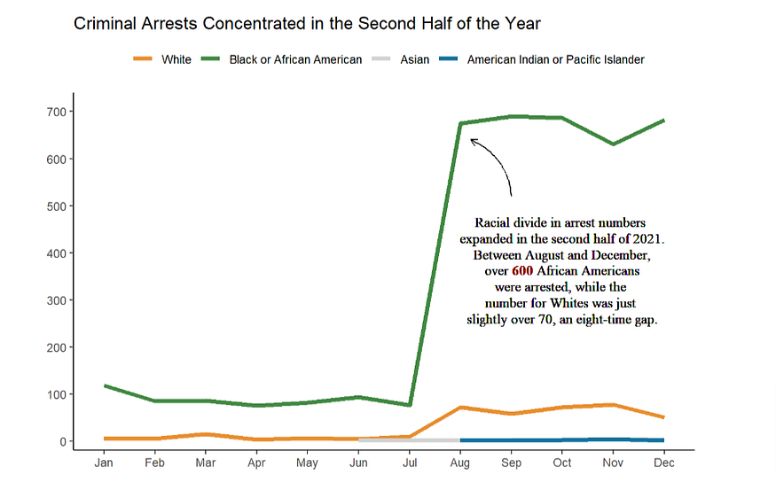
In the next section, we will focus on using the tool of explorative data analysis(EDA) to inspect our data and answer the questions I posed at the beginning of this post. We will also talk about data storytelling — the art of using data to narrate a story. Stay tuned!

Note: The blog is originally written using Quarto, the new-age Rmarkdown, and all codes can be found on my GitHub repository.

For more information about myself, feel free to check my LinkedIn page or my personal website.

Join thousands of data leaders on the AI newsletter. Join over 80,000 subscribers and keep up to date with the latest developments in AI. From research to projects and ideas. If you are building an AI startup, an AI-related product, or a service, we invite you to consider becoming a sponsor.

Published via Towards AI