Logistic Regression with BigQuery ML in 6 Steps

Author(s): Tirendaz AI

Originally published on Towards AI.

A step-by-step guide to building a logistic regression model with SQL using BigQuery ML.

Introduction

A logistic regression model is a type of statistical model that is used to predict the probability of an outcome. Logistic regression, despite its name, is a classification model rather than a regression model. The outcome is usually binary, meaning it can only be one of two possible values, such as yes or no. But logistic regression can also be easily extended to more than two classes (multinomial regression).

Here are some advantages of the logistic regression model:

• Logistic regression is easy to interpret
• It can be regularized to avoid overfitting
• Model coefficients can be interpreted as indicators of feature importance.

In this tutorial, you learn a binary logistic regression model in BigQuery ML to predict getting a tip from a customer in the Chicago taxi trips dataset. This dataset includes taxi trips from 2013 to the present, reported to the City of Chicago in its role as a regulatory agency.

Here’s what we’ll cover in this post:

• What is BigQuery?
• What is BigQuery ML?
• Creating a dataset
• Understanding the dataset
• Building a logistic regression model
• Evaluating the logistic regression model
• Making predictions using the logistic regression model

Let’s dive in!

What is BigQuery?

BigQuery is a fully-managed, serverless data warehouse that allows you to manage and analyze your data with built-in features like machine learning, geospatial analysis, and business intelligence. You can query terabytes in seconds and petabytes in minutes with BigQuery.

You can access BigQuery in the Google Cloud console interface and the BigQuery command-line tool. You can also work with BigQuery using client libraries in Python, Java, JavaScript, and Go, as well as BigQuery’s REST API and RPC API, to transform and manage data.

What is BigQuery ML?

You can use BigQuery both to query big data and to build machine learning models using standard SQL queries. The BigQuery ML lets you discover, implement, and manage data tools to make critical business decisions.

As you know, building a machine learning model on a big dataset requires extensive programming and knowledge of ML frameworks such as TensorFlow and PyTorch. BigQuery ML helps SQL practitioners to build and evaluate machine learning models using existing SQL tools and skills.

Here are some advantages of BigQuery ML:

• BigQuery ML democratizes the use of machine learning, you just need to know SQL.
• It provides a variety of pre-built models that can be used out of the box.
• You can quickly build machine learning models without exporting data from the data warehouse.
• It is easy to use and can be integrated into existing workflows.
• It is cost-effective and can be used to train models on a pay-as-you-go basis.

BigQuery Pricing

Bigquery is not free and charges you for data storage and running queries. But as part of the Google Cloud Free Tier, BigQuery provides some resources free of charge up to a specific limit. These free usage limits are available during and after the free trial period. For more information about the free usage tier, you can look here.

Logistic Regression Analysis with BigQuery in 6 Steps

Before you begin, you need to create a Google Cloud project or select a project in the Google Cloud console. Please keep in mind that after you finish your project, you can delete the project, removing all resources associated with the project.

Step 1. Create your dataset

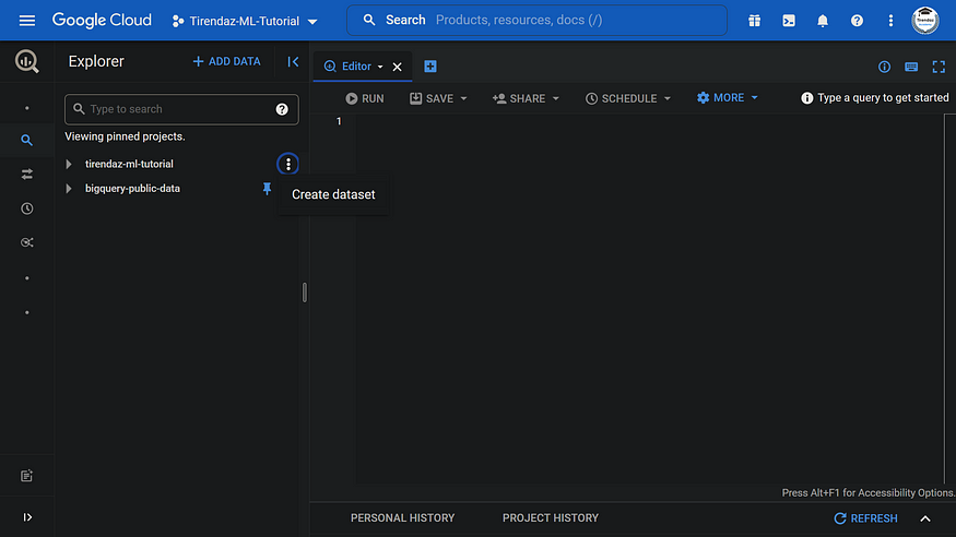
Before building the machine learning model, you need to create a dataset. To do this, let’s go to the bigquery page first. After that, click on the three dots next to the project name and then press Create dataset.

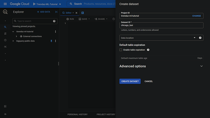
On the Create dataset page, enter a name, let’s say chicago_taxi, keeping all the other options with default values, and then click CREATE DATASET.

Step 2. Exploring the dataset

The dataset I’m going to use is the chicago_taxi_trips dataset. This dataset exists in the bigquery-public-data GCP project that hosts all the BigQuery public datasets. Let’s take a look at this dataset. Open the bigquery-public-data GCP project and find the chicago_taxi_trips dataset. After that, click on the taxi_trips table.

A new window will open showing information about the dataset.

In the schema tab, the structure of the citibike_trips table displays all the fields that can be used as labels and features.

You can also take a look at the rows of the dataset by pressing the PREVIEW tab.

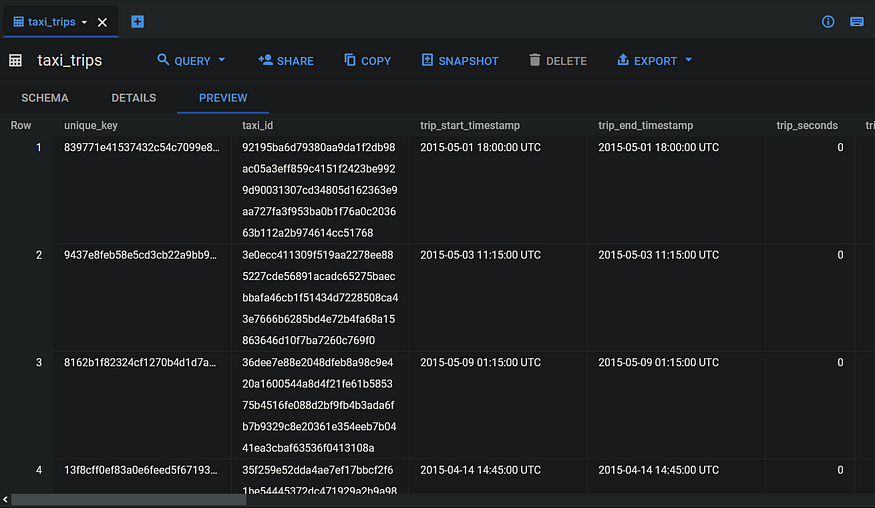
Now, to understand the dataset, let’s take a look at the first ten rows in the taxi_trips table:

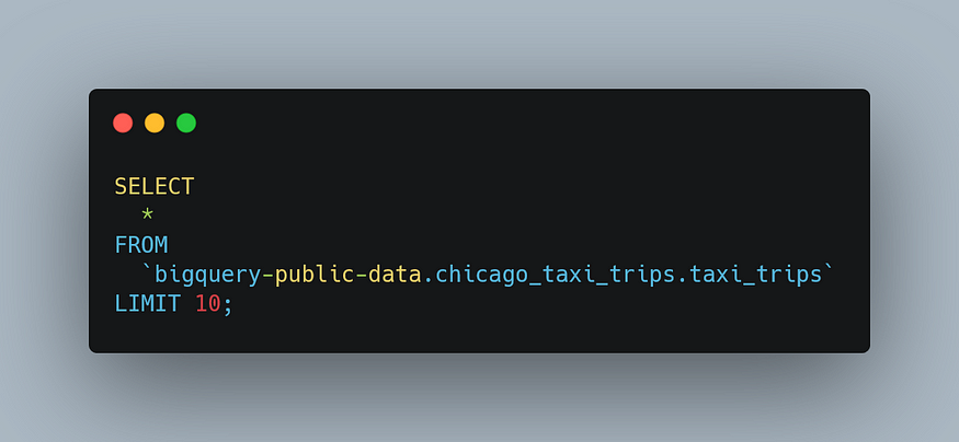
Note that I used the LIMIT 10 clause to limit the number of records in the result set. After running this query, you’ll see a screenshot like below:

Now that let’s take a look at the minimum and maximum values of the trip_start_timestamp field:

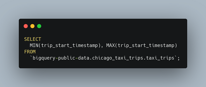
After running this query, you’ll see a screenshot like below:

As you can see, this dataset includes taxi trips from 2013 to the present. Now, let’s take a look at the missing data in the tips column:

After running this query, you’ll view a screenshot like below:

As you can see, The tips column has 7,378 missing data. Before building a machine learning model, we’ll handle these values.

Now, let’s split the dataset into three different sets: training, evaluation, and classification.

Step 3. Creating the Tables

Before training the model, the dataset is split into three sets in machine learning projects. These are the training, validation, and test sets. The model is built with the training set, the model is evaluated with the validation set, and the values in the test set are predicted with the model.

Let’s create the training table first.

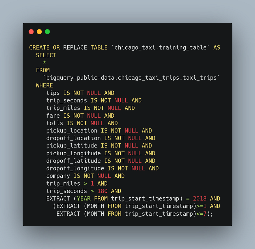
I focused on the first seven months of the 2018 year. I’m going to use the eighth and ninth months for evaluation and test tables, respectively. When you run this query, your training table is created.

Next, let’s create the evaluation table with the following query. Note that I’m going to only change the name of the table and the date.

Now let’s create the test table. This time I’m going to set the ninth month.

Awesome! We created the tables. Now, we can build the logistic regression model using the training table.

Step 4. Building the Model

You can create and train a logistic regression model using the CREATE MODEL statement with the option 'LOGISTIC_REG'. Let’s build a logistic regression model using the following query.

Here, I create the will_get_tip data. This data refers to whether the tip was received or not. If the tip is greater than zero, it’ll be coded with one, otherwise zero. I set this data to label. When running this query, you can see your model in the navigation panel. If you click tips_model, you can see the model metrics as follows:

Nice. The model metrics, such as precision, recall, and accuracy, are very high and close to the maximum of 1. The performance of the model looks good. Now, let’s evaluate the model using the evaluation table.

Step 5. Evaluating the model

After building your model, you can evaluate the performance of the model using the ML.EVALUATE function. The ML.EVALUATE function evaluates the predicted values against the actual data.

The query to evaluate the model is as follows:

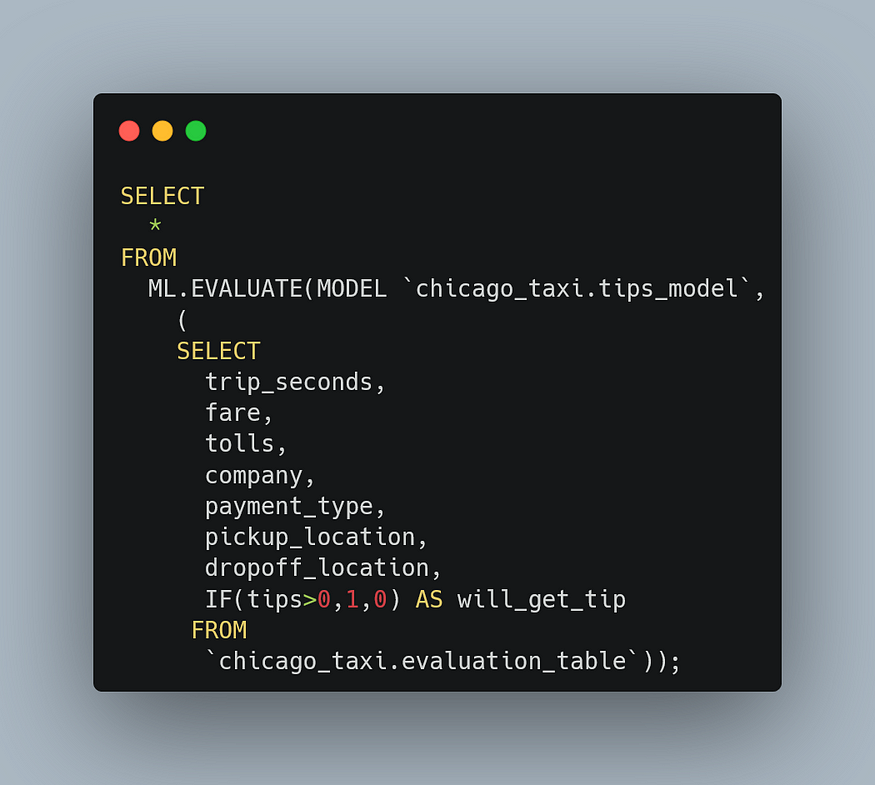
When running this query, you see the following results:

As you can see, the model metrics are very high and close to the maximum of 1. Now, let’s take a look at how to predict the test set.

Step 6. Using the model to predict the test set

After evaluating the model, the next step is to use it to predict an outcome. Let’s predict the labels using the data from the test table:

Here, I set three column, predicted_will_get_tip, predicted_will_get_tip_probs, and will_get_trip in the SELECT statement that extracts the actual and predicted values of the will_get_tip field. When you run this query, you obtain the following results.

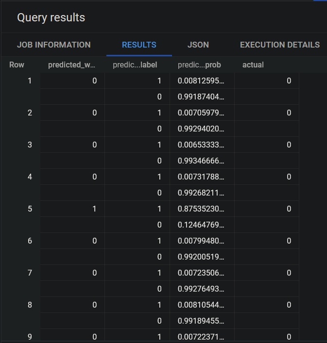
In this table, the first column contains the predicted labels, the second and third columns, respectively, the prediction labels and the probabilities of these labels, and the actual labels in the last column. Note that our model predicted almost perfectly.

Clean up

To avoid incurring charges to your Google Cloud account for the resources used in this tutorial, you can either delete the project you created or save the project and delete the dataset.

Conclusion

Logistic regression predicts the probability of an event occurring, such as a woman or a man, based on a given set of independent variables. For binary and linear classification tasks, logistic regression is a simple and more efficient method. In this post, I showed step-by-step how to perform logistic regression analysis with BigQuery ML. We first created a logistic regression model and then used this model to predict data that we did not use when building the model. It turned out that the metrics of the model we created were very high and close to a maximum of 1.

That’s it. Thanks for reading. I hope you enjoy it. Don’t forget to follow us on YouTube U+007C Instagram U+007C Twitter U+007C Linkedin U+007C Kaggle for more content on data science and cloud computing.

Hands-on Regression Analysis with BigQuery

A step-by-step guide on how to perform linear regression analysis with BiqQuery

medium.com

Data Manipulation with Pyspark in 10 Steps

I’ll guide you step by step on how to perform data manipulation with real-world data using PySpark.

levelup.gitconnected.com

If this post was helpful, please click the clap U+1F44F button below a few times to show me your support U+1F447

Join thousands of data leaders on the AI newsletter. Join over 80,000 subscribers and keep up to date with the latest developments in AI. From research to projects and ideas. If you are building an AI startup, an AI-related product, or a service, we invite you to consider becoming a sponsor.

Published via Towards AI