Medium Reader and Author Behavioural Analysis using Spacy and Seaborn in Python

Author(s): Muttineni Sai Rohith

Originally published on Towards AI.

So after my Pyspark series, I was thinking about what next to write, and after some backspaces, I thought, why not let's create something about the medium itself… And I started browsing on datasets available about medium and finally found one, On which I can use Spacy and Seaborn to do Exploratory Data Analysis.

The dataset used in this article can be found here. Unlike my previous articles where I have used Pyspark DataFrames, In this article, I will use pandas mostly, as It will be helpful for most of the readers. To implement it in Pyspark, refer to my previous articles.

Data and Objective:

This is a sample snapshot of the data. We have author, claps, reading_time, link, title, and text columns. When I wanted to apply Machine Learning to this data, two ideas struck my mind — 1. Reader and Author Behavioural Analysis, 2. Claps and Reading time prediction based on the writing pattern and topic used. I strike off the latter, as they depend mostly on the popularity of the Author — The number of followers he has and In which publication, It was posted. So let’s proceed with the first one and try to do Reader and Author Behavioural Analysis on this dataset.

Loading Data

I am going to use Pandas, and the dataset link is provided above:-

import pandas as pddf = pd.read_csv("medium_data.csv")
df.head(5)

Structuring the Data:

I said structuring here rather than preprocessing or cleaning because I am going to extract some useful information from the data, remove one Redundant column, and typecast one column.

df["len_title_words"] = pd.DataFrame([len(i.split(" ")) for i in df["title"].values])df["len_text_words"] = pd.DataFrame([len(i.split(" ")) for i in df["text"].values])

I always thought the length of the article and title plays a role in attracting readers, and I finally got a chance to test it. So we extracted that information first.

df.head(5)

Here we can see the claps column is in string format, where thousand is represented by “K”. Let's typecast that into int format.

def convert_claps(clap_values): if "K" in clap_values:
 return int((float(clap_values[:-1])*1000))
 else:
 return int(clap_values)df["claps"] = df["claps"].apply(lambda i: convert_claps(i))

I have used apply method in Pandas and converted the claps column into an int.

In our data, we have a link column, and I think, moving forward, it will not add up any information to our task. So let’s drop it.

df.drop('link', axis = 1, inplace=True)

Finally, I have structured my data and am ready to go.

Articles Analysis

I divided my Exploratory Data Analysis Into 3 sections, and Articles Analysis stands first. I am going to use Seaborn going on as Seaborn is a great library for EDA, which provides various plots to Visualize useful information from the data.

import matplotlib.pyplot as plt
import seaborn as snssns.set_theme()

Let’s Visualize the length of the articles first —

sns.displot(df['len_text_words'], color="g", legend="True", height=4, aspect=2, kde=True)
sns.rugplot(df["len_text_words"], color="r")plt.show()

Here we can see most of the articles have words between 500 to 3000.

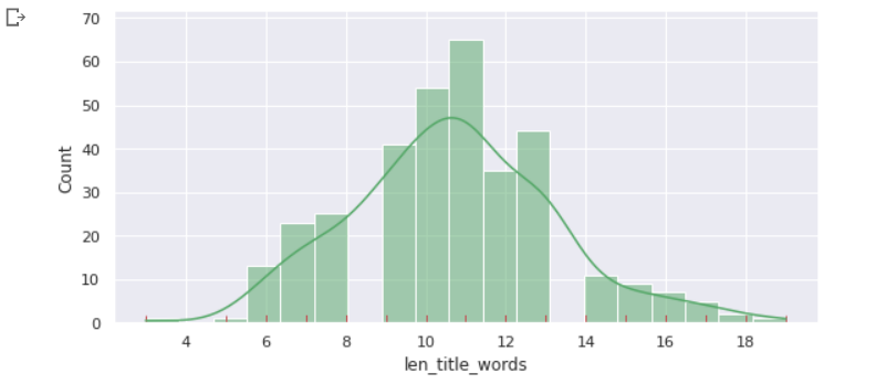
sns.displot(df['len_title_words'], color="g", legend="True", height=4, aspect=2, kde=True)
sns.rugplot(df["len_title_words"], color="r")plt.show()

We got a local maximum, ranging between 9 to 13 words, which means most of the people write titles ranging between 9 to 13 words, and Evidently, You can see my title, I belong to the same group.

sns.displot(df['claps'], color="g", legend="True", height=4, aspect=3, kde=True)
sns.rugplot(df["claps"], color="r")plt.show()

We can see that the distribution of claps is highly skewed on the right side, which clearly shows that only a few authors got a high amount of claps. It is clear that famous authors will have more claps.

From this section of the analysis, we have found that —

Mostly, the length of titles in the medium range from 9 to 13 words while the length of articles range from 500 to 3000 words

Medium Readers Analysis

We analyzed the data individually, and now let’s try to relate our data with reading time to find the reader's interests.

Now let’s also use the regplot available in seaborn — it will plot the data and a linear regression line.

sns.regplot(x = 'reading_time',y = 'claps', data=df, order=3, color="r")plt.show()

As we can see, articles with reading times ranging from 10 to 18 have more claps. So Viewers are interested to read articles that are not too short — implying they should contain useful information and not too long — which deadens the interest.

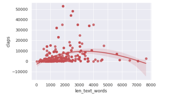
sns.regplot(x = 'len_text_words',y = 'claps', data=df, order=3, color="r")plt.show()

As we can see, there is also a slight relationship between the length of the article and the number of claps received for an article. When the Number of words in the article ranges from 1500 to 4000, There is scope for getting more claps. Keep this in mind while writing your next article.

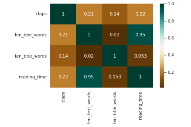
sns.heatmap(df[['claps', 'len_text_words', 'len_title_words', 'reading_time']].corr(),annot=True, cmap='BrBG')plt.show()

From the Heatmap, It is obvious that when the number of words is more, reading time is more and the length of the title has no relation to reading time and claps.

So from our analysis of the limited data we possess, We understood that —

Articles with reading times ranging from 10 to 18 have more scope to get more claps.
When the Number of words in the article are ranging from 1500 to 4000, There is scope for getting more claps.
There is no relationship between the title and the number of claps. Obviously, to get attention, the title should be attractive and catchy then lengthy.

I thought this article was becoming lengthy and maybe I could write another article about the third section but I found that I have only used 950 words, unlike the above case. So let’s proceed with the third section

Medium Authors Analysis

In this article, I will be using Spacy combined with nltk, for tokenization and predicting the Author's interest based on the most frequent words used in their Articles. To get more info on nltk, refer to my below article, where I have performed sentiment analysis using nltk.

Sentiment Analysis on OpinRank Dataset

A large amount of data that is generated today is unstructured, which requires processing to generate insights. Some…

medium.com

from collections import Counterdf['author'].value_counts()

Here we can see the Authors containing most articles in the data we possess, Let’s pick the first 3 authors and try to predict their interests in writing based on their article text.

# importing librariesimport spacy
import string
from nltk.corpus import stopwords
import nltknlp = spacy.load("en_core_web_sm")nltk.download('stopwords')

Here, we are importing nltk and spacy libraries. From spacy, we are loading the “en_core_web_sm” —which is an English multi-task CNN trained on OntoNotes.

stopwords = stopwords.words('english')
punctuations = string.punctuation

We are going to clean our data by removing stopwords and punctuation.
Stopwords — is a commonly used word (such as “the”, “a”, “an”, “in”) that a search engine has been programmed to ignore while punctuation, as we know, is symbols.

def cleanup_text(docs):
 texts = []
 for doc in docs:
 doc = nlp(doc, disable=['parser', 'ner'])
 tokens = [tok.lemma_.lower().strip() for tok in doc if tok.lemma_ != '-PRON-']
 tokens = [tok for tok in tokens if tok not in stopwords and tok not in punctuations]
 tokens = ' '.join(tokens)
 texts.append(tokens)
 return pd.Series(texts)

This method is used to remove the stop words and punctuation in the text.

def make_barplot_for_author(Author): author_text = [text for text in df.loc[df['author'] == Author]['text']]
 author_clean = cleanup_text(author_text)
 author_clean = ' '.join(author_clean).split()
 author_clean = [word for word in author_clean if word not in '\'s']
 author_counts = Counter(author_clean)
 NUM_WORDS = 25 author_common_words = [word[0] for word in author_counts.most_common(NUM_WORDS)] author_common_counts = [word[1] for word in author_counts.most_common(NUM_WORDS)] plt.figure(figsize=(15, 12))
 sns.barplot(x=author_common_counts, y=author_common_words)
 plt.title('Words that {} use frequently'.format(Author), fontsize=20)
 plt.show()

This method is used to clean the data by calling the first method and later plotting the most common words Vs. the frequency of their occurrence.

We made our code ready, now let’s focus on predicting the writing interest of 3 Authors with respect to the most used words in their articles:

Adam Geitgey

Author = 'Adam Geitgey'make_barplot_for_author(Author)

As we can see, The most frequent words are image, network, neural, learning, and face. Has he frequently written articles about images(face) using neural networks — deep learning?

Let’s check

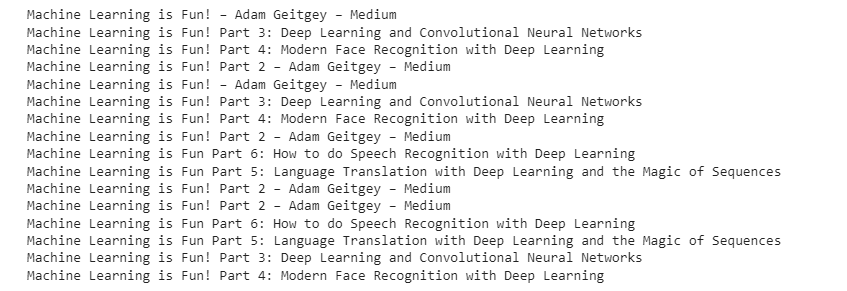
for title in df.loc[df['author'] == 'Adam Geitgey']['title']:
 print(title)

As we can see, he wrote many articles on Deep Learning and Face Recognition

Slav Ivanov

Author = 'Slav Ivanov'make_barplot_for_author(Author)

The most frequent words used are GPU, use, and CPU. In the most common words also, network, model, and learning are shown, so did he write some articles about deep learning/ neural networks on GPU?

for title in df.loc[df['author'] == 'Slav Ivanov']['title']:print(title)

As guessed, he is more interested in Deep Learning/Neural Networks and wrote two articles on GPU.

Arthur Juliani

Author = 'Arthur Juliani'make_barplot_for_author(Author)

The most commonly used words are q, network, action, state, agent, reward, and learning…. Being a person who worked for 3 years in Reinforcement learning, I can easily guess he is talking about Reinforcement learning.

Let’s check:

Gotcha…

So we are able to predict the Author’s interest based on the most common words they have used.

And now I also fall in the category of Authors whose words range from 1500 to 4000.

Stay tuned for my upcoming articles….

Happy coding….

Join thousands of data leaders on the AI newsletter. Join over 80,000 subscribers and keep up to date with the latest developments in AI. From research to projects and ideas. If you are building an AI startup, an AI-related product, or a service, we invite you to consider becoming a sponsor.

Published via Towards AI