The Unsung Hero of Machine Learning — Linear Algebra

Author(s): Saif Ali Kheraj

Originally published on Towards AI.

Machine learning, data mining, deep learning, and advanced optimization algorithms all rely heavily on linear algebra. In this post, we will go over some of the most fundamental concepts, including Gaussian elimination, Inverse matrices, and the concept of linear dependence and independence. First and foremost, I would like to provide motivation. Linear algebra is widely used in almost all machine learning algorithms. For example, in Machine Learning, it is used in algorithms such as Linear Regression to find the best-fit parameters for predictive modes. For example, Gaussian elimination aids in the solution of normal equations derived from the least squares method. In operations research, Gaussian elimination is used in simplex algorithms to solve optimization problems. Optimization and numerical analysis in operations research, machine learning, and deep learning are three major areas where Linear Algebra is used.

Operations Research (OR): In linear programming, Gaussian elimination is used in the simplex algorithm to solve optimization problems. For example, allocating resources in the most efficient way for vaccine delivery or to solve public health problems.

Data Science: Gaussian elimination can be used for feature selection by identifying linearly dependent features that can be removed to simplify models.

Deep Learning: In deep learning, particularly in the training of neural networks, backpropagation algorithms involve computations that can be viewed as sophisticated extensions of Gaussian elimination for solving systems of equations.

Reinforcement Learning: Solving Markov Decision Processes in reinforcement learning often requires working with transition matrices and reward functions, where linear algebra and the concept of independence play a key role.

Systems of Linear Equation Intuition and Graphical Methods

Let us see Linear equation with n=2

The goal in solving a system of linear equations is to find the values of the variables that satisfy all the equations in the system. These solutions can be visualized as the points of intersection of the lines. Let us illustrate this through an example:

Let us pick simple 2 equations

Graphical Method — Intersection

If we graph this equation, we get

Thus, we have solutions where 2 lines intersect, which is 4 and -1.

Graphical Method — Column View

Let us now look at it a bit differently using column view.

We can rewrite the equation as:

Here, the goal is to look at some combination of the column vectors on the left side to produce one on the right side.

Let us see the column view in the graph. We have 2 vectors right over here: one is (2,1), which is indicated by a red line, and the other is (1,-2), which is indicated by the orange line. We need to scale these two vectors so that when we add them, the resultant vector is (7,6), as indicated by the green line. As shown here, we must scale the red vector four times and the orange vector one time in the negative direction. This is represented by a dotted line of red and orange. When we add these two, we get a green resultant vector (7,6). As you can see above, adding scaled orange and red yields (7,6) via black dotted lines.

Thus, we may have to lengthen, shorten, or combine vectors to arrive at the destination vector.

This is the underlying idea behind solving linear equations. We will look at more complex equations to solve a system of linear equations using matrix operations.

Solving Systems of Linear Equations through Matrix Operations

We can use the same concept in three dimensions, but three dimensions and beyond are difficult to visualize and solve graphically.

Due to the three-dimensional nature of this example, each equation is represented by a hyperplane rather than a line. The resulting solution or point of intersection will be a line.

The column view is the same as I described above. We still need to find a combination of x, y, and z to create the final vector.

If we have hundreds of constraints or variables, we must devise a nice solution. We can use a very nice method known as Gaussian Elimination to solve system of linear equations.

Gaussian Elimination — (Unreduced Row Echelon Form)

We essentially converted the above column view(Figure 5) into this nice matrix(Figure 6) so that we can easily solve Gaussian elimination. Finally, we must end up with a triangular matrix to identify pivots. Let’s take a step-by-step look at how we can make it triangular before determining the values of x, y, and z.

First, we need to get rid of x from the second and third rows. To make it zero, we can add and subtract or do other operations. Let us see.

Here R1 represents Row 1, R2 represents Row 2, R3 represents Row 3. We are essentially doing addition subtraction operations to make it work.

As you can see above, we were able to make the second and third rows 0. We now need to eliminate y from the third row.

Here, we have created a nice triangular matrix. We now have three pivots: 1, -2, and -5. Now that we have completed forward elimination, we can use back substitution to determine the values of x, y, and z. We start from the last row.

Then we substitute z into 2nd equation to get y:

Now that we have z and y, we can use it to solve the first equation:

We now have 3 parts, which are our x,y, and z. Here, we made use of forward elimination to get the triangular system, and then we worked through back substitution further to get the final solution. However, it is possible to reduce the operations involved in back substitution by performing additional row operations to transform the matrix from the echelon form (current form) to the reduced echelon form.

Reduced Echelon Form

A matrix is in reduced echelon form when each column that contains a nonzero entry (usually made to be 1) has zeros not just below that entry but also above that entry.

A matrix is in reduced echelon form when each column containing a nonzero entry (usually set to 1) has zeros both below and above that entry.

Reduced Echelon Form Property

1. Leading Ones: Each non-zero row starts with a 1, called a leading 1 (pivot), which is the first non-zero element in the row.
2. Staircase Pattern: The leading 1s move to the right as you move down the rows, creating a staircase pattern.
3. Above and Below Zeros: Every element in a column above and below a leading 1 is zero.
4. Normalized Rows: Each pivot is in a column where all other elements are zeros, and the row containing the pivot has been normalized so that the pivot itself is 1.
5. Row Reduced: The matrix has undergone row reductions to the point where no further simplification is possible

What we solved above was in Echelon form, which we then solved with back substitution. We can now use the matrix we left above to create what we see on the right side (Reduced echelon Form). As you will see, once we have it in reduced echelon form, there is no need for back substitution.

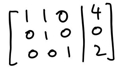
We started with the echelon form provided above. Now, let’s set the pivot entries to 1 and the rest to 0.

For the second row, divide by -2 to make the leading coefficient 1, and for the third row, divide by -5 to make the leading coefficient 1

Let’s use a very simple operation to eliminate 1 in the first row, third column, and -1/2 in the second row.

Now we just need to eliminate 1 in the first row thats it.

The matrix is now in reduced row echelon form (REF). The solutions to the system are:

We solved it without the need for back substitution. Thus, the system of equations has been solved, and the Gauss-Jordan elimination is complete.

Thus, if we have n equations, we will have n pivots. In this case, we will say that the system of equations is nonsingular. However, keep in mind that the complexity of solving a system of linear equations using Gaussian elimination is high to the power of 3.

Matrix Inverse

Now you understand how Gaussian elimination and Guass-Jordan elimination work. Let us go a step further and study invertible matrices. In Linear Algebra, an invertible matrix is one with an inverse. Matrix A is invertible if there is another matrix A^-1, or you may call any other name, such that multiplying A with A^-1 gives the identity matrix I. Identity is a special matrix with 1s on the diagonal, as we saw above when solving the Gauss-Jordan elimination.

To find A’s inverse from A, we will use the previously discussed Gauss-Jordan elimination.

So we need to essentially convert the left side part to the right side to get A inverse.

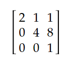
Let us consider the matrix

Let’s say we want to find its inverse; we will use the above-mentioned format.

We will now use different operations similar to the one used above to make the left-hand side equal to the identity matrix, resulting in all of the elements on the main diagonal being 1 and all of the other elements being 0.
Once the left side equals the identity matrix, the right side becomes our inverse matrix.

I will not solve it here, but you should find the final solution listed below:

These are the key concepts to remember in Linear Algebra. It is not always possible to transform the left-hand side, A, into an identity matrix. If A can be converted into an identity matrix, we say it is non-singular, which means we can find the inverse. In advanced terminology, nonsingular denotes invertibility. To summarize, we have two things to remember:

Non-singular (invertible): A matrix that can be converted into the identity matrix using row operations and thus has an inverse.
Singular (non-invertible): A matrix that cannot be transformed into the identity matrix using row operations and lacks an inverse.

Linear Independent and Linearly Dependent

Let us now proceed to our final section, where we will understand Linearly dependent and Linearly Independent in a very simple manner. In layman’s terms, if we have three vectors and we can create a third vector from the two we already have, we say they are linearly dependent.

For example, consider the vectors x1, x2, and x3. If we can use x1 and x2 in some combination to create a third vector, then these vectors are linearly dependent.

Similar to what we solved above, we will use the same approach but only create the first two vectors to solve for the last. Then, we can apply a system of linear equations. If, for example, when solving systems of linear equations, we get a matrix like this:

This is impossible as w1.x1 + w2.x2 cannot be equal to 1(last row). Thus, these vectors are linearly independent.

If the last row would have been all 0s, then this would have been linearly dependent.

Conclusion

These concepts are important and serve as the silent engine behind the scenes of various AI and ML algorithms. Understanding its principles and application is not only beneficial but also required for anyone seeking to make informed decisions based on quantitative data.

References:

[1] https://www.cliffsnotes.com/study-guides/algebra/linear-algebra/linear-systems/gaussian-elimination

[2] https://online.stat.psu.edu/statprogram/reviews/matrix-algebra/gauss-jordan-elimination

[3]https://www.blacksacademy.net/texts/LinearDependenceIndependenceSingularAndNonSingularMatrices.pdf

[4] https://en.wikipedia.org/wiki/Invertible_matrix

Join thousands of data leaders on the AI newsletter. Join over 80,000 subscribers and keep up to date with the latest developments in AI. From research to projects and ideas. If you are building an AI startup, an AI-related product, or a service, we invite you to consider becoming a sponsor.

Published via Towards AI