How to make a GAN to generate color images.

Author(s): Pere Martra

Originally published on Towards AI.

In this article, we continue our journey through the exciting world of GANs and learn how Generative AI works with a Color Dataset.

In the first article, we saw how to create a DCGAN for the MNIST Dataset. That is, 28 × 28 images in Grayscale. The complexity of the dataset will be increased slightly in this step, and we will use Cifar-10. It is also a well-known dataset, in fact, it is one of the Datasets that come with Keras. Contains six thousand 32 × 32 color images.

They are slightly larger images than the ones used in the first article, but the most important difference is the color.

If you have come to this article looking for a tutorial on how to create a simple GAN, don’t worry, you don’t have to read the previous article. Stay here.

I am going to start by giving some common explanations to understand how a GAN works. Then we will see the code in parts and explain it. Finally, we will have the complete code of the GAN.

Those of you who have already read the first article and do not want to go over how a GAN works again, can go directly to the section: What else will we see?

The code is available at Google Colab & Kaggle:

GAN Tutorial 2. Generating color images

Explore and run machine learning code with Kaggle Notebooks U+007C Using data from No attached data sources

www.kaggle.com

Google Colaboratory

Edit description

colab.research.google.com

You have all the Notebooks in the GAN Series in a repository in gitHub under a MIT License. Feel free to clone it, and don’t forget to watch or star it if you want to receive the updates and new notebooks.

GitHub — peremartra/GANs: GAN tutorials using TensorFlow, Keras & Python

GAN tutorials using TensorFlow, Keras & Python. Contribute to peremartra/GANs development by creating an account on…

github.com

A brief overview of how a GAN works.

A GAN is a neural network, usually used to generate images, composed of two networks: a Generator and a Discriminator.

The Generator receives an input of data, which is simply noise. Random data ordered in a Gaussian form. Do not worry that it is just a call to a function. With this input, it generates an output in the format of the image we want to create.

Let’s generate the noise to use as input for the Generator model:

test_noise = tf.random.normal([16, 100])

This call returns the noise we can use for the generator. We are telling it to return an array of 16 rows with 100 values each. The generator will use these 16 rows to make 16 different images from the data with 100 length values. That is, a row is needed for each image to be generated.

The size of the noise does not have to be 100. It is an arbitrary value, some of the most used values ​​are: 50, 100, 128, 1024…

The best study to date on the input noise of a GAN is the one carried out in 2020 by Manisha Pandala, Denoit Das, and Sujit Gujar: Effect of input noise dimension in GANs.

The study shows that for images like those from the Cifar-10 Dataset, there are no differences between a value of 100 and one of 900, but that with small values, like 2 or 10, quality and variety in the images are lost.

The other model that is part of the GAN is the Discriminator. This is responsible for deciding when an image belongs to the Original Dataset or is a False image created by the Generator. The discriminator receives an image, in this case with the format 32 × 32 × 3, and has a Boolean output that indicates when the image is authentic or false.

Both models are trained together, and they modify their weights depending on the ability of the discriminator to guess which images are true or fake.

The generators’ intention is to create images that fool the discriminator. The discriminator wants to always be able to tell which images came from the generator.

What else are we going to see in this article?

For those of you who have already read the first article, I will explain a little about what we will see next.

• Larger images are used, so the input and upsampling of the generator are changed.
• Color images. The output of the generator is modified and obviously the input of the discriminator.
• We are going to create two functions that will allow us to create flexible GAN structures.
• We will use the tag smoother. One of Soumith Chintala’s GAN Hacks.

Create the Generator for color images.

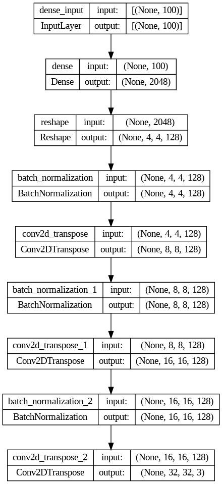
The Generator model transforms the input data as it passes through the model layers. So, the noise that has been used as input, of a predetermined length, ends up being a 32 × 32 × 3 image at the output of the model.

To accomplish this, we will first have a Dense layer, which will receive the input data and which must have enough nodes to contain a reduced version of the image to be generated. But because we want the model to be able to quickly learn on each step of each epoch, we’ll size it to contain X versions of the thumbnail.

keras.layers.Dense(4 * 4 * 128, input_shape=[noise_input], 
 activation=keras.layers.LeakyReLU(alpha=0.2)),
keras.layers.Reshape([4, 4, 128]),

In the generator that we are going to see, the first dense layer will have enough nodes to contain 128 × 4 × 4, that is, 2048 data. In a second layer, we change the shape so that it adapts to the shape we need to contain these reduced images.

Let’s say we want to make the final result 32 × 32 × 3, and for now, we have a shape of 4 × 4 × 128.

From this point, an upsampling process must be carried out until the format of the image is reached.

keras.layers.Conv2DTranspose(128, kernel_size=4, strides=2, padding="SAME", 
 activation=keras.layers.LeakyReLU(alpha=0.2)),
keras.layers.BatchNormalization(),

I execute this process with a Conv2DTranspose layer. That layer doubles the size of the image. By having the strides parameter informed with the value 2, the data is multiplied by 4, and in this first pass we would go from having a shape of 4 × 4 = 16, to a shape of 8 × 8 = 64.

After the Conv2DTranspose layer, I use a BatchNormalization layer. This layer gives stability to the system. It normalizes the output from the previous layer before passing it to the next one.

A LeakyReLU layer is being used as an activator, inside the Conv2DTranspose layer. We could really use it as an outer layer and place it behind the BatchNormalization layer in order to receive the normalized output.

An alternative structure could be:

#Another possible options to perform the upsampling. 
keras.layers.Conv2DTranspose(128, kernel_size=4, strides=2, padding="SAME"),
keras.layers.BatchNormalization(),
keras.layers.LeakyReLU(alpha=0.2), 

However, I have not noticed a difference in the quality of the generated images for the cifar-10 dataset. I don’t think we can find any performance differences either, so it’s up to everyone’s preference to use LeakyReLU as a separate layer or as an activator in Conv2DTranspose.

In the final generator, this upsampling process will have to be repeated three times, so the image goes from a 4 × 4 size to a 32 × 32 size.

To finish the model, we need a layer whose output matches the shape of the image that will be generated.

#Last layer
keras.layers.Conv2DTranspose(3, kernel_size=4, strides=2, padding="SAME",
 activation='tanh'),
 ])

I have taken advantage of the last layer, Conv2DTranspose to give the necessary shape to the output. Maybe a most common solution is to use a Conv2D layer to format the output, and keep the Conv2DTranspose layer to do the Upsample with a higher number of nodes.

#An alternative to the final layers of the Generator. 
keras.layers.Conv2DTranspose(128, kernel_size=4, strides=2, padding="SAME", 
 activation=keras.layers.LeakyReLU(alpha=0.2)),
keras.layers.BatchNormalization(),
keras.layers.Conv2D(3, kernel_size=5, activation='tanh', padding='same')

In both alternatives, the activator for the last layer is tanh, whether we use a Conv2DTranspose or a Conv2D layer. This activator gives us an output range of -1 to 1, the same range we used to normalize the input. It is one of the recommendations that can be found in the GAN Hacks.

It’s time to put it all together and look at the generator code I used for the GAN.

noise_input = 100

generator = keras.models.Sequential([
 keras.layers.Dense(4 * 4 * 128, input_shape=[noise_input], 
 activation=keras.layers.LeakyReLU(alpha=0.2)),
 keras.layers.Reshape([4, 4, 128]),
 keras.layers.BatchNormalization(),

 #First UpSample doubling the size to 8x8
 keras.layers.Conv2DTranspose(128, kernel_size=4, strides=2, padding="SAME", 
 activation=keras.layers.LeakyReLU(alpha=0.2)),
 keras.layers.BatchNormalization(),

 #Second UpSample doubling the size to 16x16
 keras.layers.Conv2DTranspose(128, kernel_size=4, strides=2, padding="SAME", 
 activation=keras.layers.LeakyReLU(alpha=0.2)),
 keras.layers.BatchNormalization(),

 #Last UpSample doubling the size to 32x32, and shaping the output. 
 keras.layers.Conv2DTranspose(3, kernel_size=4, strides=2, padding="SAME",
 activation='tanh'),
 ])

Above you can see the code of the generator, with its input layer, the main body where the upsamples are made, and its output layer.

As you can see, I’m using the same number of nodes in the two Conv2DTranpose layers. A common practice is to reduce the number of nodes as upsampling is performed. But in this specific case, since I take advantage of the last Conv2DTranspose layer as the output layer and its nodes have already been reduced enough, it is not necessary to reduce them in the previous layers.

At the end of the article, you can see a generator that reduces the number of nodes between upsamplings. In the Colab notebook, and in Kaggle, you can find the two generators, and compare the quality of the generated images.

Some of the recommendations known as GAN hacks have been used in the generator:

• The use of LeakyReLU.
• The use of BatchNormalization layers.
• I’m using a kernel_size divisible by strides.
• Use tanh activator on the last layer.

In conclusion, a simple generator has been created, but it is highly optimized for the data set used.

Create the GAN discriminator.

The discriminator will be responsible for identifying which image is real and which is not. It will receive an image as input and the output will be a binary.

The Discriminator is simpler than the Generator. Instead of upsampling, it will downsize the data using Conv2D layers. To finally flatten the data with a Flatten layer and pass the result to the Dense layer that will decide if the data belongs to a real or fake image.

discriminator = keras.models.Sequential([
 keras.layers.Conv2D(64, kernel_size=5, strides=2, padding="SAME",
 activation=keras.layers.LeakyReLU(0.2),
 input_shape=[32, 32, 3]),
 keras.layers.Dropout(0.4),

 keras.layers.Conv2D(64, kernel_size=3, strides=2, padding="SAME",
 activation=keras.layers.LeakyReLU(0.2)),
 keras.layers.Dropout(0.4),

 keras.layers.Conv2D(64, kernel_size=3, strides=2, padding="SAME",
 activation=keras.layers.LeakyReLU(0.2)),
 keras.layers.Dropout(0.4),
 
 keras.layers.Flatten(),
 keras.layers.Dense(1, activation="sigmoid")

The first convolutional layer of the model receives the data with the shape 32 × 32 × 3. While the output is made by a single node Dense layer, with a sigmoid activation. That ensures us to obtain a 0 or a 1 as a result.

As you can see, I have used three layers of Dropout, with a fairly high rate of 0.4. I use it so that the discriminator doesn’t fit too well with the current data in the dataset to prevent it from becoming too good at identifying which images are authentic and which are fake. Which could make it hard for the generator to produce images that could fool the discriminator.

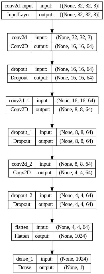
In each of the convolutional layers, the output is reduced by half. With what, we pass from the 32×32 of the first layer to 4×4×64 of the last one before flatten the data with a Flatten layer.

I have maintained the number of nodes in the convolutional layers, although it is a common practice to increase it as data size is reduced. As with the generator, we find an example at the end of the article, in the notebook in Colab and in Kaggle, where I increase the number of nodes and we can compare the result.

Function to train the GAN.

Now that we have the two models, the generator and the discriminator, we need to build a function that uses them together to train the GAN and make images that can be taken as authentic.

The code, and, therefore, the explanations to be given, are 95% identical to those of the first series of the GAN series:

Creating our first optimized DCGAN

The following article is the first in a series that will discuss generative adversarial networks. Let’s get started…

pub.towardsai.net

I recommend that you go through him to obtain more details about the training function. But if you don’t have time, or just don’t want, do not worry, I’m going to explain the basics.

We can find two large blocks in the function, one to train the discriminator, and the other to train the GAN.

In the first block we train the discriminator and for this we pass a set of data formed by generated images and by images of the dataset, with their respective labels. To train the discriminator, we call its Train_on_batch function, making sure that their layers can be trained by putting the discriminator.trainable to True.

In the second block we go on to train the generator, for this it is called the Train_on_batch function of the GAN. We pass a block of false images generated by the generator, but labeled as if they were true images. Before calling the GAN function train_on_batch, we have to make sure that we have marked the discriminator layers as non-trainable. When using the GAN, the generator will train depending on the success it has in deceiving the discriminator. That is why we are interested in only being able to modify the weights used in the layers of the Generator, since we have already trained the discriminator in the previous step.

The main difference with the previous article is that in this one I have used what is called a label softener. That is, instead of marking all the labels as 0 if they are false or 1 if they are true, some ranges have been used. Fake labels are marked with values between 0 and 0.3, while true ones will have values between 0.8 and 1.2.

To smooth the labels, I have used these two functions:

def smooth_positive(y):
 return y -0.2 + (np.random.random(y.shape) * 0.4)

def smooth_negative(y):
 return y + np.random.random(y.shape) * 0.3

The values for smoothing are within the recommended ranges in the GAN Hacks, although I have slightly reduced them. There is discussion about whether to soften only the positive labels or to do it also with the negative ones, I have chosen to smooth both.

def train_gan(gan, dataset, random_normal_dimensions, n_epochs=30):
 #Get the GAN layers. 
 generator, discriminator = gan.layers

 for epoch in range(n_epochs):
 print("Epoch {}/{}".format(epoch + 1, n_epochs)) 
 for real_images in dataset:
 # Calculate the batch_size
 batch_size = real_images.shape[0]

 # FIRST PHASE: TRAINING THE DISCRIMINATOR. 
 # Noise that we are going to use as input for the Generator. 
 noise = tf.random.normal(shape=[batch_size, random_normal_dimensions])

 # Creating fake images with the Generator. 
 fake_images = generator(noise)

 # concat fake and real images. 
 mixed_images = tf.concat([fake_images, real_images], axis=0)

 # Labels for the Discriminator. 
 # 0 / 0.3 for fake images. 
 # 0.8 / 1.2 for real images. 
 discriminator_zeros = smooth_negative(np.zeros((batch_size, 1)))
 discriminator_ones = smooth_positive(np.ones((batch_size, 1)))
 discriminator_labels= tf.convert_to_tensor(np.concatenate((discriminator_zeros, discriminator_ones)))

 # Mark the Discriminator layers as trainables. 
 discriminator.trainable = True

 # Call train_on_batch with images and labels. 
 discriminator.train_on_batch(mixed_images, discriminator_labels)

 # SECOND PHASE: TRAINING THE GENERATOR. 
 # Creamos el ruido que servirá como entrada de la GAN
 noise = tf.random.normal(shape=[batch_size, random_normal_dimensions])
 
 # Create "Real" labels for fake images. 
 generator_ones = smooth_positive(np.ones((batch_size, 1)))
 generator_labels = tf.convert_to_tensor(generator_ones)

 # Freeze the discriminator labels. 
 discriminator.trainable = False

 # Train the GAN with noise and labels. 
 gan.train_on_batch(noise, generator_labels)
 
 #Print the images each epoch
 plot_results(fake_images, 8) 
 plt.show() 

With this, we already have almost everything, the auxiliary functions to print the images, the loading of libraries are missing, but all this can be found in the notebook in Google Colab, and Kaggle.

At the moment we can see the result and compare it with the images of the original Dataset.

It seems clear that our Generator is understanding the kind of images that the discriminator is looking for, and that as the epochs progress it is getting more refined images.

It is possible that the generator is managing to fool the discriminator more and more, but, with few exceptions, I don’t think they will be able to fool a human. We know that within each Cifar-10 Image there is a recognizable object in the real world, which can be a car, an animal, a truck… any element that belongs to one of the Cifar-10 categories.

Functions to create a Generic Generator and discriminator.

In these first two articles of the GAN series, we have observed that the skeleton of the generator and the discriminator have been very similar. A different number of upsizings and a different input and output have been required. But the base is the same.

It seems clear that the creation of the Generator and the discriminator can be encapsulated in two functions.

def adapt_generator(initial_0, initial_1, nodes, upsamplings, multnodes = 1.0, endnodes = 3, input_noise=100):
 #initial_0, initial_1: size of the initial mini image. 
 #nodes: nodes in the first Dense layers. 
 #upsamplings: number of upsamplings bucles. 
 #multnodes: a multiplicator to modify the nodes in each upsampling bucle. 
 #endnodes: nodes of the last layer. 
 #input_noise: size of the noise. 

 model = keras.models.Sequential()

 #First Dense layer. 
 model.add(keras.layers.Dense(initial_0 * initial_1 * nodes, input_dim=input_noise, 
 activation=keras.layers.LeakyReLU(alpha=0.2)))
 model.add(keras.layers.Reshape([initial_0, initial_1, nodes]))
 model.add(keras.layers.BatchNormalization())

 #Upsampling bucles. 
 nodeslayers = nodes
 for i in range(upsamplings-1):
 nodeslayers = nodeslayers * multnodes
 model.add(keras.layers.Conv2DTranspose(nodeslayers , kernel_size=4, strides=2, padding="SAME", 
 activation=keras.layers.LeakyReLU(alpha=0.2)))
 model.add(keras.layers.BatchNormalization())

 #last upsample and last layer. 
 model.add(keras.layers.Conv2DTranspose(endnodes, kernel_size=4, strides=2, padding="SAME", 
 activation='tanh'))
 
 return model

The function to create the Generator has the parameters:

• the initial mini image size
• The number of nodes in the first layer.
• The number of upsamplings to perform (each upsampling doubles the size of the image)
• A multiplier to vary the number of nodes.
• The nodes of the last layer.
• The size of the noise used as input for the first dense fall.

I’m going to create a Generator for an input of4 x 4 with a first Dense Layer with 128, 3 upsamplings, an output of 3, and I’m going to reduce a 50% the nodes in each upsamplig.

adapt_gene = adapt_generator(4, 4, 128, 3, multnodes = 0.5)

As we have indicated a value of 0.5 in multnodes, the nodes are reduced by half in each iteration of upsampling.

The function for the discriminator is similar:

def adapt_discriminator(nodes, downsamples, multnodes = 1.0, in_shape=[32, 32, 3]):
 #nodes: nodes in the first Dense layers.
 #downsamples: number of downsamples bucles. 
 #multnodes: a multiplicator to modify the nodes in each downsample bucle.
 #in_shape: Shape of the input image. 

 model = keras.models.Sequential()
 
 #input layer % first downsample 
 model.add(keras.layers.Conv2D(nodes, kernel_size=5, strides=2, padding="SAME",
 activation=keras.layers.LeakyReLU(0.2),
 input_shape=in_shape))
 model.add(keras.layers.Dropout(0.4))
 
 #creating downsamples
 nodeslayers = nodes
 for i in range(downsamples - 1):
 nodeslayers = nodeslayers * multnodes
 model.add(keras.layers.Conv2D(nodeslayers, kernel_size=3, strides=2, padding="SAME",
 activation=keras.layers.LeakyReLU(0.2)))
 model.add(keras.layers.Dropout(0.4))
 
 #ending model
 model.add(keras.layers.Flatten())
 model.add(keras.layers.Dense(1, activation="sigmoid"))
 
 return model

The discriminator function allows us to indicate:

• The nodes in the initial layer.
• The number of downsamples we want.
• A multiplier to modify the number of nodes in each downsample.
• The input Shape.

We are going to create a Discriminator with 64 nodes in the first layer, 3 downsamples loops, and double the number of nodes in each loop.

 adapt_disc = adapt_discriminator(64, 3, multnodes = 2)

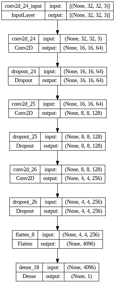
The number of nodes is duplicated in each upsample.

The creation of the GAN, the training and compilation would be the same as for the Generator and Discriminator created in the traditional way.

It seems to me that the result with these second models has been better than with the first. Therefore, the use of node reduction in the generator and the increase in the discriminator have provided good results. The most important improvement is seen with the images generated with 30 epochs.

With 100 epochs of training, figures begin to appear in the content of the images. In three of them a vehicle could be guessed, and some figures could be confused with animals.

I think we’ve done a good job.

What have we learned?

We have used a new dataset that asked us to perform a different number of Upsamples than the one performed in the previous article. So, I hope that it has become much clearer for us how the main structure of a GAN is built.

Taking advantage of the fact that we already have it clear, we have encapsulated it in a couple of functions. That allows us to create different GAN models that adapt to different datasets, changing only the parameters of the functions.

We have also used a new GAN Hack: the smoothing of the labels of the images used.

What’s next?

We have two new functions that allow us to create Generators and Discriminators, and they could be used to create a model that works with the MNIST Dataset. It can be a good exercise to practice by yourself with simple DCGANs.

We are just at the beginning of this journey. The next Dataset contains images that can still be considered small, but that are already double those used up to now.

There is still a lot to come, and we are going to see more complex GAN models such as conditional GANs.

I write about TensorFlow and machine learning regularly. Consider following me on Medium to get updates about new articles. And, of course, You are welcome to connect with me on LinkedIn.

More articles in the GAN series:

Pere Martra

GANs From Zero to Hero

View list4 stories

If you like TensorFlow and want to know some interesting techniques, check my series: TensorFlow Beyond The Basics.

Pere Martra

TensorFlow beyond the basics

View list3 stories

Join thousands of data leaders on the AI newsletter. Join over 80,000 subscribers and keep up to date with the latest developments in AI. From research to projects and ideas. If you are building an AI startup, an AI-related product, or a service, we invite you to consider becoming a sponsor.

Published via Towards AI