How to Achieve Effective Exploration Without the Sacrifice of Exploitation

Last Updated on June 23, 2020 by Editorial Team

Author(s): Sherwin Chen

Machine Learning

A gentle introduction to the Never Give Up(NGU) agent

Modern deep reinforcement learning agents often do well in either exploration or exploitation. Agents like R2D2 and PPO can easily achieve super-human performance on games with dense rewards, but they generally fail miserably when the reward signal becomes sparse. On the other hand, exploration methods such as ICM and RND can effectively learn in sparse reward environments at the cost of performance in dense reward ones.

We discuss an agent, namely Never Give Up(NGU) proposed by Puigdomènech Badia et al. at DeepMind., that achieves state-of-the-art performance in hard exploration games in Atari without any prior knowledge while maintaining a very high score across the remaining games. In a nutshell, the NGU agent uses 1)a combination of episodic and life-long novelties to encourage the agent to visits rarely visited states, whereby achieving effective exploration; 2)the framework of Universal Value Function Approximator(UVFA) to enable the agent to simultaneously learn different trade-offs between exploration and exploitation.

This post consists of two parts: Firstly, we discuss how the NGU agent computes intrinsic rewards that motivate it to effectively explore the environment. Secondly, we discuss the whole agent, seeing how it utilizes UVFA to learn both exploratory and exploitative policies.

Intrinsic Rewards

Limitations of Previous Intrinsic Reward Methods

It is known that naive exploration methods, such as 𝝐-greedy can easily fail in sparse reward settings, which often require courses of actions that extend far into the future. Many intrinsic reward methods have been proposed lately to drive exploration. One type is based on the idea of state novelty which quantifies how different the current state is from those already visited. The problem is that these exploration bonus fades away when the agent becomes familiar with the environment. This discourages any future visitation to states once their novelty vanished, regardless of the downstream learning opportunities it might allow. The other type of intrinsic reward is built upon the prediction error. However, building a predictive model from observations is often expensive, error-prone, and can be difficult to generalize to arbitrary environments. In the absence of the novelty signal, these algorithms reduce to undirected exploration schemes. Therefore, a careful calibration between the speed of the learning algorithm and that of the vanishing rewards is often required.

The Never-Give-Up Intrinsic Reward

Puigdomènech Badia et al. propose an intrinsic reward method that combines both episodic and life-long novelties as follows

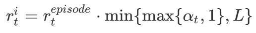
In the above equation, the episodic novelty encourages visits to states that distinct from the previous states but rapidly discourage revisiting the same state within the same episode. On the other hand, the life-long novelty regulates the episodic novelty by slowly discouraging visits to states visited many times across episodes. We address how each novelty is computed in the following subsection.

Episodic novelty module

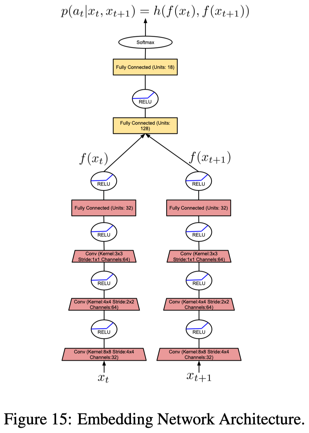
In order to compute the episodic intrinsic reward, the agent maintains an episodic memory M, which keeps track of the controllable states in an episode. A controllable state is a representation of an observation produced by an embedding function f. It’s controllable as the function is learned to ignore aspects of an observation that are not influenced by an agent’s actions. In practice, NGU trains through an inverse dynamics model, a submodule from ICM that takes in observations x_t and x_{t+1} and predicts action a_t​ (see Figure 15 on the left). The episodic intrinsic reward is then defined as

where n(f(x_t))​ is the counts for visits to the abstract state f(x_t)​. We approximate these counts​ as the sum of the similarities given by a kernel function ​K over the content of the memory M​. In practice, pseudo-counts are computed from the k​-nearest neighbors of state f(x_t)​ in the memory M​ with the following inverse kernel

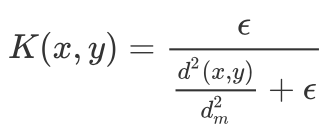
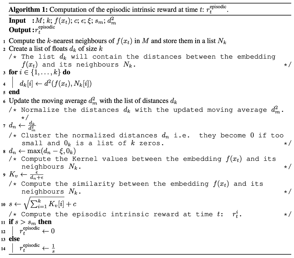
where 𝝐 guarantees a minimum amount of “pseudo-counts”, d is the Euclidean distance and d²_m is the running average of the squared Euclidean distance of the k-nearest neighbors. This running average is used to make the kernel more robust to the tasks being solved, as different tasks may have different typical distances between learned embeddings. Algorithm 1 details the process

Life-long novelty module

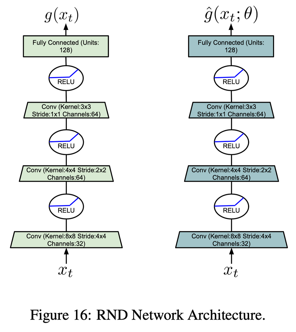
Puigdomènech Badia et al. uses the RND to compute the life-long curiosity, which trains a predictor network \hat g​ to approximate a random network g​. The life-long novelty is then computed as a normalized mean squared error:

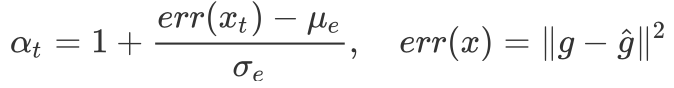
The following figure demonstrates the RND architecture used by the agent

The Never-Give-Up Agent

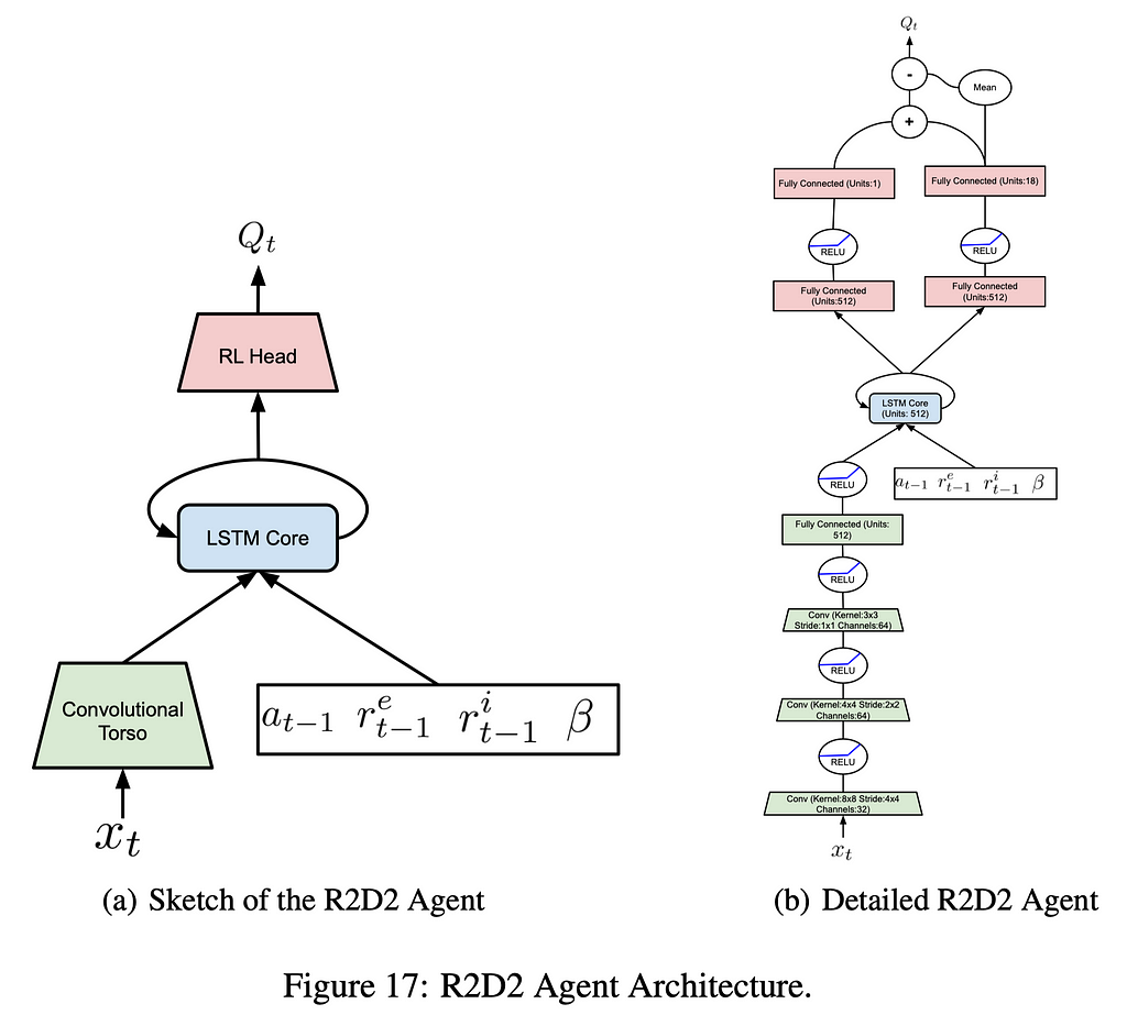
As shown in Figure 17, the NGU agent uses the same architecture as the R2D2 agent, except that it additionally feeds intrinsic reward r^i and their coefficient 𝛽 to the LSTM. This scheme, following Universal Value Function Approximator(UVFA), allows the agent to simultaneously approximate the optimal value function with respect to a family of augmented rewards of the form

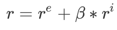
where r^e is the extrinsic reward provided by the environment, r^i is the intrinsic reward defined in the previous section. The reward, as well as the policy, is parameterized by a discrete value 𝛽 from the set {𝛽_j}_{j=0}^{N-1}, which controls the strength of r^i. This allows the agent to learn a family of policies that make different trade-offs between exploration and exploitation.

The advantage of learning a larger number of policies comes from the fact that exploitative and exploratory policies could be quite different from a behavior standpoint. Having a larger number of policies that change smoothly allows for more efficient training. One may regard jointly training the exploration policies, i.e. 𝛽>0​, as training auxiliary tasks, which helps train the shared architecture.

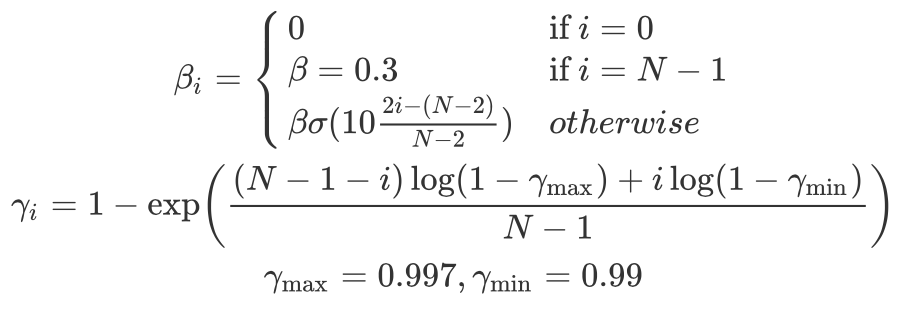
In practice, we additionally associate the exploitative policy(with 𝛽=0) with the highest discount factor 𝛾 and the most exploratory policy(with the largest 𝛽) with the smallest discount factor 𝛾. We use smaller discount factors for exploratory policies because the intrinsic reward is dense and the range of values is small, whereas we would like the highest possible discount factor for the exploitative policy in order to be as close as possible to optimizing the undiscounted return. The following equations show the schedule Puigdomènech Badia et al. use in their experiments.

Reinforcement learning objective

As the agent is trained with sequential data, Puigdomènech Badia et al. use a hybrid of Retrace(𝝀​) and the transformed Bellman operator. This gives us the following transformed Retrace operator

Like DDQN, we compute this operator using the target network and update the online Q network to approach this value.

References

Badia, Adrià Puigdomènech, Pablo Sprechmann, Alex Vitvitskyi, Daniel Guo, Bilal Piot, Steven Kapturowski, Olivier Tieleman, et al. 2020. “Never Give Up: Learning Directed Exploration Strategies,” 1–28. http://arxiv.org/abs/2002.06038.

---

How to Achieve Effective Exploration Without the Sacrifice of Exploitation was originally published in Towards AI — Multidisciplinary Science Journal on Medium, where people are continuing the conversation by highlighting and responding to this story.

Published via Towards AI