Tesla’s Self Driving Algorithm Explained

Author(s): Inez Van Laer

Originally published on Towards AI the World’s Leading AI and Technology News and Media Company. If you are building an AI-related product or service, we invite you to consider becoming an AI sponsor. At Towards AI, we help scale AI and technology startups. Let us help you unleash your technology to the masses.

On Tesla AI Day, Andrej Karpathy — the director of AI and Autopilot Vision at Tesla — enlightened us with a presentation about their self-driving neural network. To save you time, I have outlined the general concepts so you get a sense of how intelligent Teslas truly are.

💡 You can view the full video on Youtube.

Version 1

At the start of autonomous driving development, the main objective was to let the car move forward within a single lane and keep a fixed distance from the car in front. At that time, all of the processing was done on an individual image level.

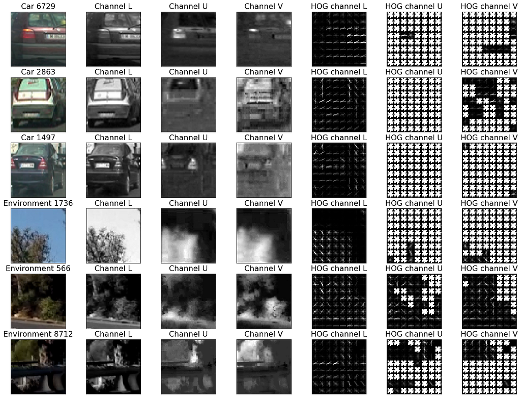
So how can we detect cars or lanes in images?

The Feature Extraction Flow or Neural Network Backbone

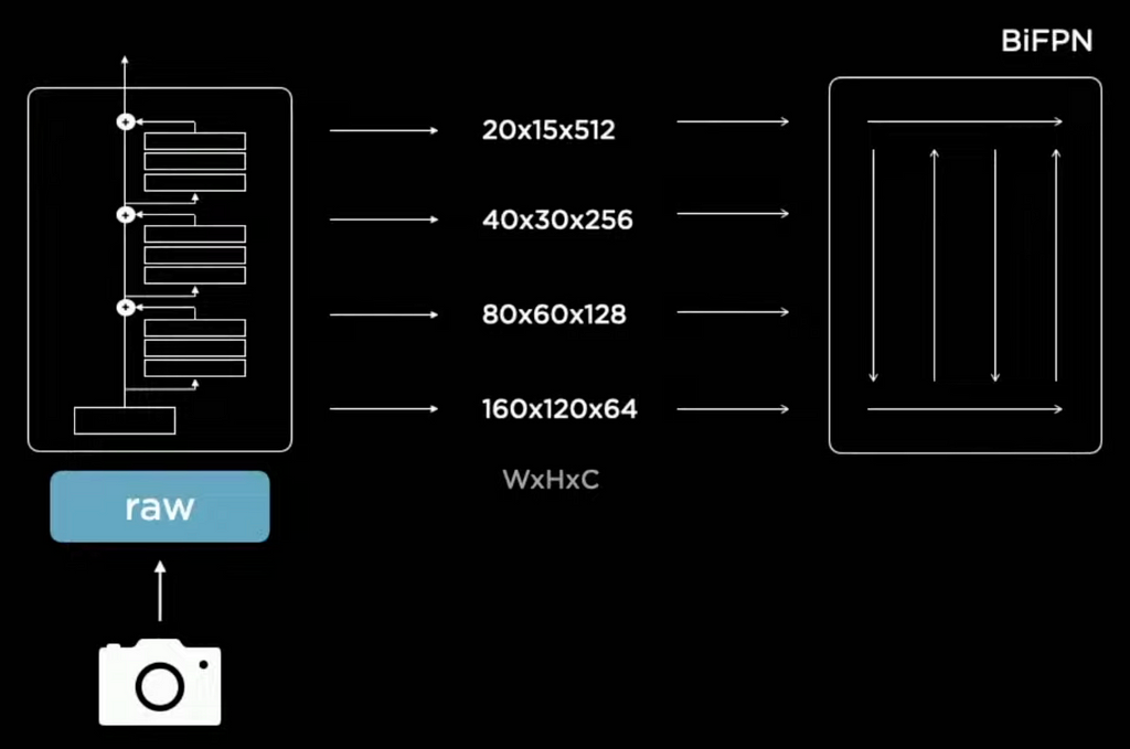
The raw images of the car camera are processed by a residual neural network (RegNet) that extracts multiple blocks or feature layers in width (W) x height (H) x channel (C).

The first feature output has a high resolution (160 x 120) and focuses on all the details in the image. Moving all the way to the top layer, with a low resolution (20 x 15) but with a greater channel count (512). Intuitively, you could visualize each channel as a different filter that activates certain parts of the feature map or image, for example, one channel puts more emphasis on edges and another on smoothing parts out. Therefore, the top layer puts more focus on the context by using a variety of channels. Whereas, the lower layer focuses more on the details and specifics by using a higher resolution.

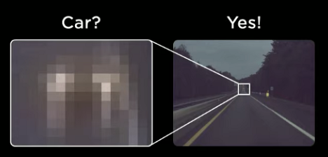
The multiple feature layers interact with each other via a BiFPN, a weighted bi-directional feature pyramid. For example, the first detailed layer thinks it sees a car but is not sure. At the top of the feature pyramid, the context layer provides feedback that the object is at the end of the road. So yes it is probably a car, but it is blurred out due to the distance.

Multi-Task Learning 💪🏽

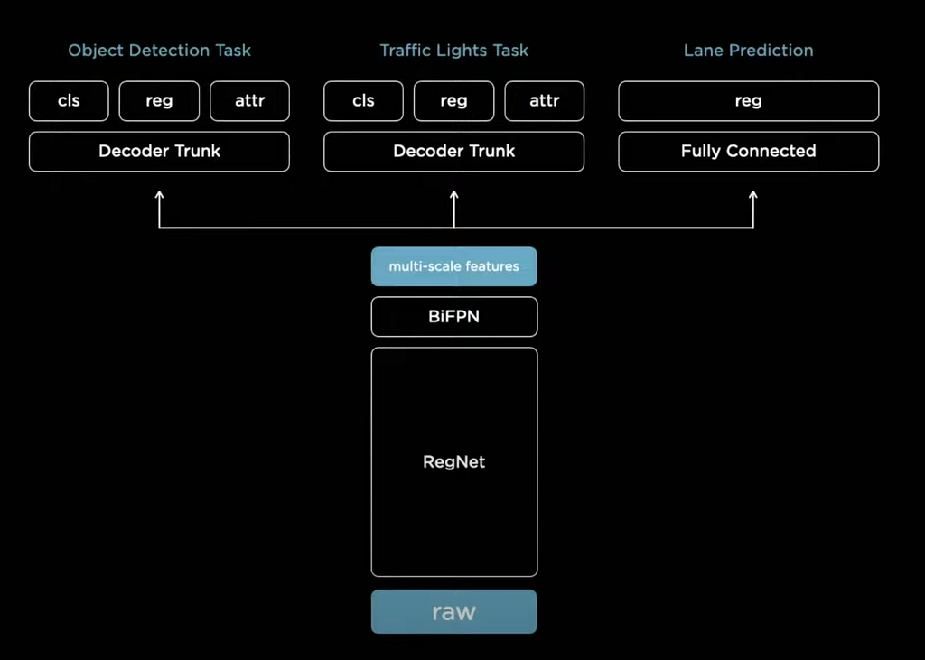
The output features are not only used to predict cars but are used for multiple tasks such as traffic light detection, lane prediction, etc. Each specific task has its own decoder trunk or detection head, which is trained separately, but they all share the same neural network backbone or feature extraction mechanism. This architectural layout is called a HydraNet.

So, why this HydraNet?

1. Feature Sharing — It is more computationally efficient to run a single neural network backbone.
2. Decouple Tasks — You can fine-tune tasks individually without affecting other predictions. This creates more robustness.

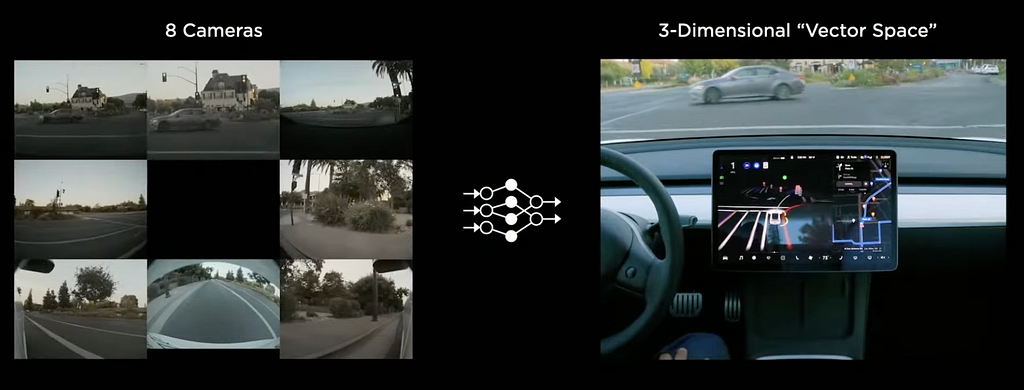
Now that we understand how the network works for individual images, we can ask ourselves, how do we combine multiple images into a 3D space? After all, we want to have a thorough understanding of the surroundings, especially if the car is self-driving.

Stitching Images

Tesla’s engineer developed an occupancy tracker in order to stitch all the camera images together. Despite the effort, they quickly realized that tuning the occupancy tracker and all of its hyperparameters was extremely complicated. Lane detection looked great on the image but when you cast it out into a 3D space it looked terrible.

How do you transform features from image-space to vector-space?

Version 2

Multi-Scan Vector Space Prediction

Instead of stitching the images explicitly by hand, you want them to be part of your neural network, which will be trained end-to-end. The image space predictions should be mapped on a raster with a top-down view.

The first challenge is that the road surface could be sloping up or down and there could be occlusions due to cars passing by.

So how do you learn a model to overcome visual barriers?

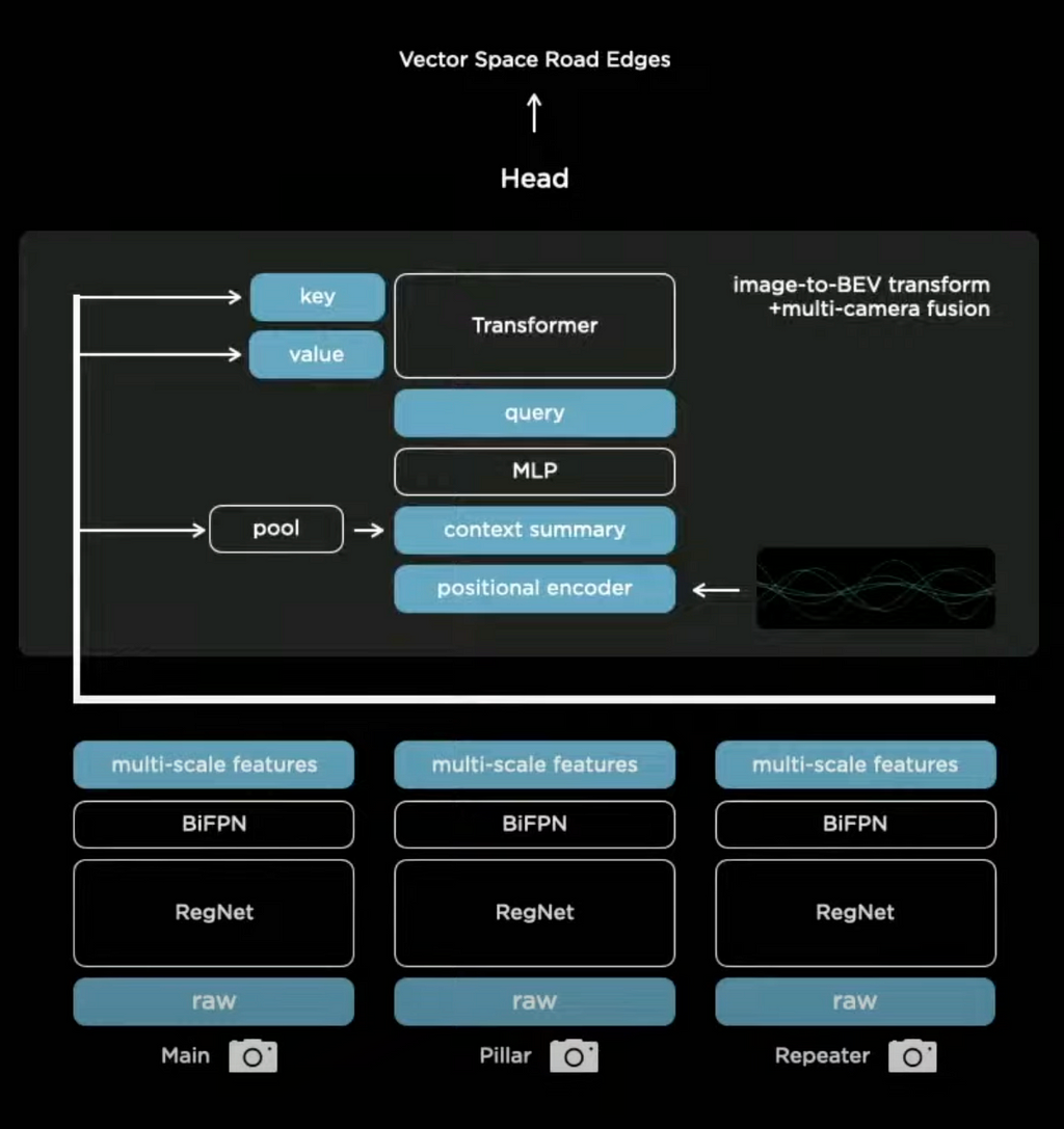
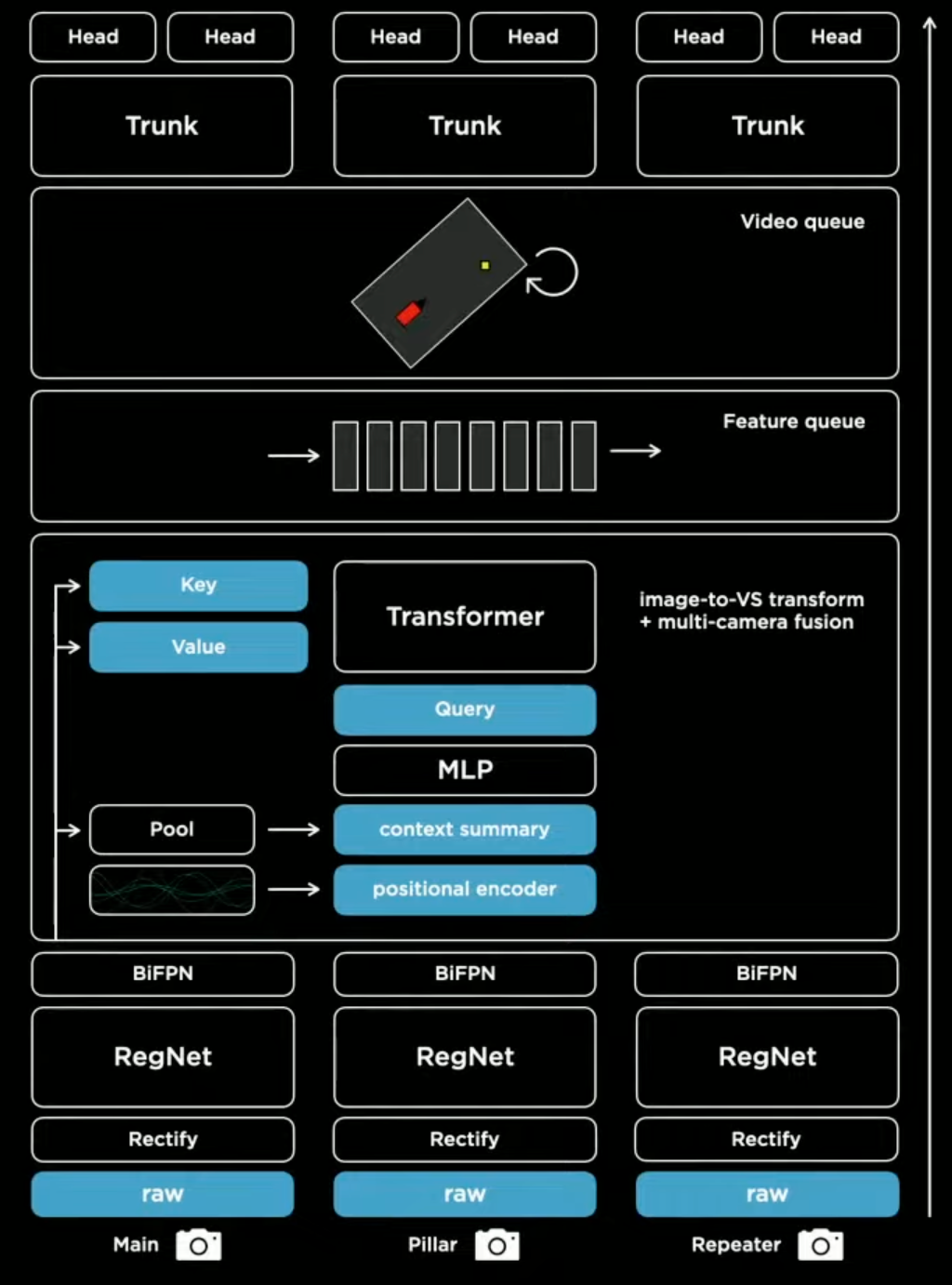
If there is a car occluding a viewpoint you want to learn to pay attention to different parts of the image. To accomplish this, a transformer with multi-headed self-attention is used.

To get a better understanding of transformer models, you can read the paper: Attention Is All You Need (arXiv)

Essentially how it works is that a raster is initialized with the size of the real-world output space (vector space). The yellow pixel, at a known position in that output space, will ask the neural network with the 8 cameras for information about that pixel — the query. The keys and the queries interact multiplicatively and then the values get pulled accordingly. After some processing, the output will be a set of multicam features about that pixel that can be used for predictions. To make this work, precise calibration and good engineering are key.

How do you handle variations in camera calibration?

Rectify to a Common Virtual Camera

If you build a car, the cameras will always be positioned in a slightly different way. Before you feed images into the neural network, you need to calibrate the camera first. The most elegant way to do this is to transform all of the images into a synthetic virtual camera using a rectification transform. This is a method of camera calibration that translates all of the images into a common virtual camera.

The final result is a big performance improvement and better predictions coming directly out of the neural network. After we have the image prediction right, we still need to consider another dimension — time.

Adding Time to the Equation

There are a large number of predictions that need time or video context. For example, if you want to identify whether a car is parked or traveling. If it is traveling, how fast is it going? If you want to predict the road geometry ahead, the road markings 50 meters ago can be helpful, etc.

How do we include time in the network?

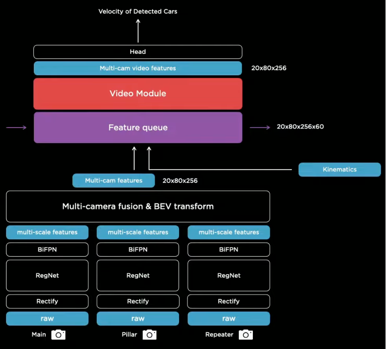
Feature Queue Module

Multiscale features are generated by the transformer module and are concatenated with kinematics, such as velocity and acceleration, as well as the tracking of the position of the car. These encodings are stored in a featured queue which is then consumed by a video module.

When do we push to the feature queue?

Time-based Queue

The latest features are pushed to the queue within a specified timeframe of milliseconds. If a car gets temporarily obstructed, the neural network can look at the memory and reference it in time. Therefore, it can learn that something is occluded at a certain point in time.

Space-based Queue

In order to make predictions about the road geometry ahead, it is necessary to read the line marks and road signs. Sometimes they occur a long time ago and if you only have a time-based queue you may forget the features while you’re waiting behind a red light. In addition to a time-based queue, there is a space-based queue, and information is pushed every time the car travels a certain fixed distance.

Video Neural Network 🎥

The feature queue is consumed by a spatial recurrent neural network (RNN). The RNN keeps track of what’s happening at any point in time and has the power to selectively read and write to the memory or cached queue. As the car is driving around only the parts that are near the car and where the car has visibility are updated. The result is a two-dimensional spatial map of the road with channels that track different aspects of the road.

Putting Everything Together

First, the raw images are passed through the rectification layer, to correct for camera calibration. Then the images are passed to the residual network to process them into features at different scales and channels. The features are fused into multi-scale information through a transformer module to represent it in vector space. The output space is pushed into a featured queue in time or space that gets consumed by a video module like the spatial RNN. This video module then continues into the branching structure of the hydranet with trunks and heads for all the different prediction tasks.

💡 Elon Musk announced that Tesla is going to hold a second AI Day on August 19, 2022.

Thanks for reading this post on Tesla’s autopilot. I hope it helped you to understand the general concepts of Tesla’s autopilot. More details can be found in Jason Zhang’s Medium blog post Deep Understanding Tesla FSD Series.

---

Tesla’s Self Driving Algorithm Explained was originally published in Towards AI on Medium, where people are continuing the conversation by highlighting and responding to this story.

Join thousands of data leaders on the AI newsletter. It’s free, we don’t spam, and we never share your email address. Keep up to date with the latest work in AI. From research to projects and ideas. If you are building an AI startup, an AI-related product, or a service, we invite you to consider becoming a sponsor.

Published via Towards AI