Self-Supervised Learning and Transformers? — DINO Paper Explained

Author(s): Boris Meinardus

Originally published on Towards AI.

How the DINO framework achieved the new SOTA for Self-Supervised Learning!

Transformers and Self-Supervised Learning. How well do they go hand in hand?

Some people love the Transformer architecture and welcome it into the computer vision domain. Others don’t want to accept that there is a new kid on the playground.
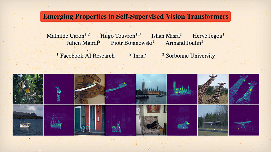
Let’s have a look at what happens when you build on BYOLs [2] idea of self-distillation in self-supervised learning and plug in a Vision Transformer! This is what the authors at Facebook AI Research asked themselves when working on the first DINO [1] paper. Are there any cool emerging properties when combining both? Well, one cool effect of using Transformers is the ability to look at the model’s self-attention maps!

That is what we see here in the teaser image above. We can visualize the self-attention map of the class token of the final layer and pretty much see that the model learns to recognize the main object in the image. The model pretty much learns a segmentation map without any labels!

I think this is really cool!!!

When predicting the final representation of the first image in the first row, the model pays the most attention to the bird, when doing so for the first image in the second row, it pays attention to the boat, and so on!
This boat example could be especially tricky when training in a supervised fashion since that model is more inclined to learn shortcuts, like also paying attention to the water because water and a metal object mean boat.

But before we continue with the cool findings, let’s have a look at how they achieved all this!

The DINO framework

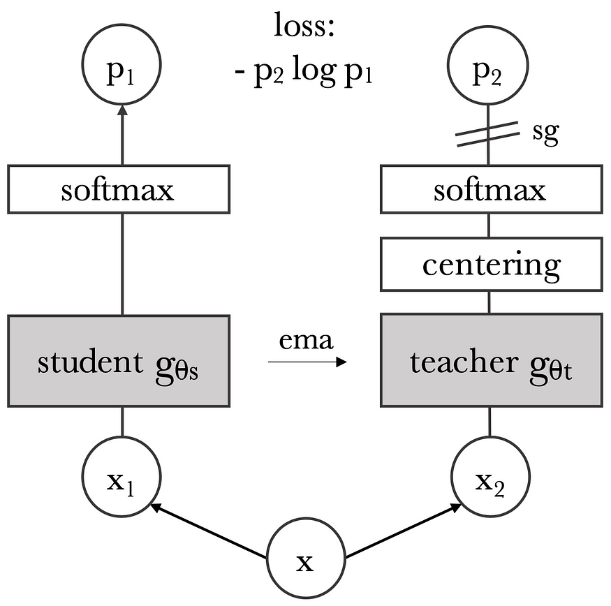
This is the training pipeline which is also part of the Self-distillation family.

We once again have our original source image, apply two different sets of random augmentations, and end up with two different views, x1 and x2. We again have our online network, which is now called the student network, and our target, now called the teacher network, which once again is an exponential moving average of the student network.
From here on, things start to look different. We have NO further projection layer NOR a prediction head! If there is no prediction head, how do we prevent (or rather reduce the likelihood of) representation collapse? Well, first of all, we have this centering right here, which can be seen as simply adding a bias c to the teacher predictions.

This bias uses batch statistics to compute the mean of the batch and is updated similarly to the EMA.

This hyperparameter m is pretty much the same as the ???? parameter in the EMA equation. We update the bias parameter c slightly with every batch. This centering is probably the main operation to avoid collapse to a constant function! Centering prevents one dimension from dominating as a kind of pseudo-label but also encourages collapse to the uniform distribution! That is why the framework also somewhat relies on the sharpened softmax since it has the opposite effect.

Imagine you have a bunch of pictures, and you want to teach the model to recognize different objects in those pictures. Now, if the model always pays attention to the same object because it gets its attention the most, like a cute dog, the model will only learn about dogs and not anything else. Centering is like trying to be fair and making sure that the AI learns about all the different objects equally. It’s like saying, “Okay, let’s divide the pictures into different groups, and each group should be looked at equally.” This way, the model will learn about different objects in a balanced way. The model is encouraged to learn about a variety of features or different “pseudo-classes” rather than focusing on a single dominant feature/class. Sharpening, on the other hand, is a technique used to make sure that when wanting to “classify” an object, i.e., wanting to move the whole feature vector strongly along one feature dimension, the model doesn’t get confused and always picks different objects randomly, i.e., simply always predicts a uniform distribution. It’s like making sure that each time the model does tend to pick an object, it’s confident and sure about its choice. After applying the far less sharpened softmax function to the student output, the final loss is the cross entropy loss.

And why cross entropy and not the MSE like in BYOL?

If we look at row 2, the MSE surprisingly does work with DINO but cross entropy (rows 1, 3, 4) simply seems to work better.
DINO also works when adding a further prediction head to the student network (row 3)! But that doesn’t seem to help much either.
In fact, we don’t even necessarily need the softmax operations if we use the MSE loss. But if we use cross entropy, we obviously do because that loss is defined over probability distributions, which, again, seems to work better!

Okay… That was a lot to unpack and somewhat build intuition! But this hopefully shows how much experimentation is done to see what empirically works and what doesn’t!

Loss function

What also seems to work better is not simply using the cross entropy over all different view embeddings but using a very specific setup!

Let’s see what this actually means and return to our friendly little quokka!

Let’s again generate multiple views; this time, let’s say 4. Change their color slightly, and crop and resize. Now, when cropping, we want to specifically have two cases, crops that contain 50% or more of the original image and crops with smaller cutouts. These large crops are called global crops, marked with the “g”.

When assigning our views to the two branches, for the teacher, we specifically want to only use our global views, and for the student, we’ll use all views, i.e., the local and global crops.

What we are now comparing is the teacher embedding of one of the global crops and all the embeddings of all samples from the student network, except for the embedding of the same global view. We can now compute the cross entropy of each student embedding with this one teacher embedding and repeat this whole process.
Voila, we have our weird-looking cross-entropy loss that enforces local-to-global correspondence.

We already talked about the two cropping cases in the SimCLR post, where we have two adjacent views and the here enforced case of local and global views. Apparently, the model learns better when learning to look at smaller parts of a bigger object and when trying to match it to its embeddings. The embedding of the global view has more information at hand and can thus better recognize the object.

Building intuition

This assumption makes sense to me, as long as the teacher produces better embeddings than the student and is also made assumed in the BYOL paper, but since the authors of DINO went ham on experiments, ablation studies, and the quest of building intuition, they actually verified this assumption by looking at the accuracy of both student and teacher networks during training.

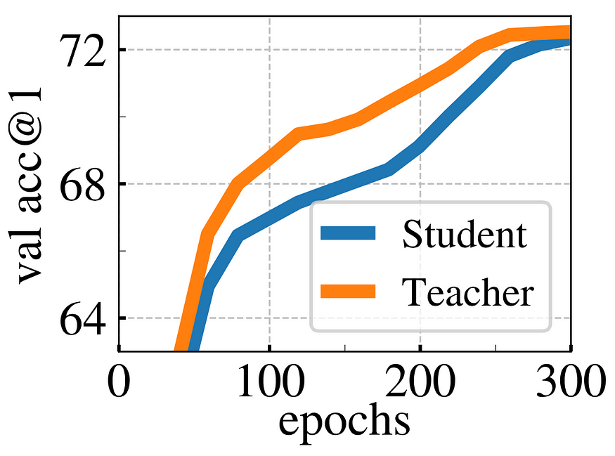
The teacher does appear to be smarter than the student and whenever the student improves, the teacher does so as well, since it is a more stable version of the student. Keyword: exponential moving average. All that up to a certain point, where the teacher doesn’t have anything to teach anymore, and both converge.

But okay, cool. We just looked at the novel and improved self-distillation framework that, once again, is agnostic of the architecture. So, where are the transformers, and why are they specifically so special with this framework?!

Let’s simply look at a comparison between different Self-Supervised learning frameworks and plug in the classic ResNet and a Vision Transformer.

When looking at the validation accuracy of the trained ResNets, we can see that the DINO framework yields the best performance but can rather be considered on par with the other baseline approaches.

However, when replacing the ResNet architecture with a Vision Transformer, DINO unleashes its potential and outperforms the other baselines significantly! Especially in the case of k-NN classification. K-NN is one of the standard evaluation protocols for Self-Supervised learning in today’s time but it wasn’t back then when SimCLR and BYOL were developed and published.

Sigh… Back then… As if that wasn’t like 2–3 years ago…

K-NN!
Why is it so cool and how does it work? You don’t need any fine-tuning!

We still need labels, obviously, but we now simply project all our labeled data into our representation space to generate our class clusters.

When wanting to classify a new data point, e.g., an image, we pass it through our Neural Network and project it into representation space. We then simply count the k nearest neighbors (in this case, 3) and do a majority vote. In this case, most of our neighbors are of class orange, so the new image is also classified as class orange. This k is a new hyperparameter (as if there weren’t enough already) and, in the paper, is found to yield the best results when set to 11.

Results

Okay, cool. Here is a table with super exciting results. DINO, of course, is the best when looking only at ResNets, only at ViTs, and across different architectures. But looking at same-sized architectures, it’s still not beating a fully supervised model.

Cool. But even cooler is again looking under the hood and visualizing the attention maps.

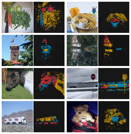
When looking at those from the top 3 attention heads, we can see impressive properties! Similar to CNNs, where each kernel is responsible for extracting certain features, we can see that different attention heads pay attention to different semantic regions of an image! In the first example on the second row, one head pays attention to the clock face, one to the flag, and one to the tower itself! Or, one row below that example, we can again see how one head focuses on the collar, one on the head, and one on the white neck of the zebra!

Isn’t this so cool?!

All of this is learned without any labels, without any specific segmentation maps!
In fact, we could simply interpret one attention map as a segmentation output and compare supervised and Self-Supervised training using DINO!

As already mentioned, when training in a self-supervised fashion, the model learns to focus more on the main object in the image than when training a network specifically for classification.

The learning signal is stronger in the case of self-supervised learning!

In classification, the model can learn to use shortcuts to solve its task. When trying to match the image of the bird to the bird class, the model can use the sky or the branches as important features.
In the end, if the classification accuracy, or rather the loss that is optimized, is satisfied, the model doesn’t really care, whether it actually only looks at the bird or also its surroundings. In Self-supervised training, on the other hand, we don’t really have such a simple and straightforward optimization task. The model needs to learn to match color-augmented, local views to global views. It has to learn to produce embeddings while ignoring all augmentations applied to the original source image. The features it needs to learn to extract are much more specific.

I hope that makes sense, even though your brain might be somewhat overwhelmed with all this information especially if you have just read all my previous posts on self-supervised learning!
I mean… my brain was fried after doing all this research. And I probably didn’t even get all the details!

Self-supervised learning is really cool, powerful, and interesting! But all this was just scratching the surface! Further advancements, e.g., Masked Image Modeling, were used by the follow-up papers to DINO, iBOT [3], and DINOv2 [4]. The learned representations can be used for so many different downstream tasks!

The training and architecture improvements of DINOv2 over iBOT are a list of many small, tuned knobs like the right patch size, teacher momentum, a better centering algorithm, and so on.

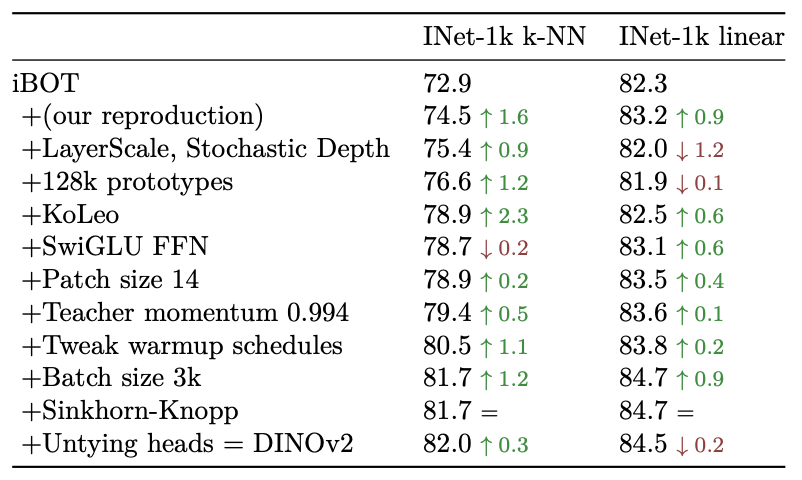
Also, DINOv2 developed a very sophisticated data preprocessing pipeline to generate a much larger, but curated dataset.

Self-Supervised Learning remains a daunting field with a mind-boggling array of methods each with intricate implementations. That’s why Meta AI recently published a 45-page long cookbook [5] to help navigate through this field. So, if you are interested in this topic (and since you are still reading at this point, you probably are) I can highly recommend you have a look at the publication. It is a lot, but a very good read! And I hope this little series will have helped you to get a fundamental understanding that will also aid you in navigating the cookbook.

Thank you very much for reading!
If you haven’t already, feel free to check out my other posts to dive deeper in Self-Supervised Learning and the latest AI research.

P.S.: If you like this content and the visuals, you can also have a look at my YouTube channel, where I post similar content but with more neat animations!

References

[1] Emerging Properties in Self-Supervised Vision Transformers, M. Caron et. al, https://arxiv.org/abs/2104.14294

[2] Bootstrap your own latent: A new approach to self-supervised Learning, J. B. Grill, F. Strub, F. Altché, C. Tallec, P. H. Richemond et al., https://arxiv.org/abs/2006.07733

[3] iBOT: Image BERT Pre-Training with Online Tokenizer, J. Zhou et al., https://arxiv.org/abs/2111.07832

[4] DINOv2: Learning Robust Visual Features without Supervision, M. Oquab, T. Darcet, T. Moutakanni et al., https://arxiv.org/abs/2304.07193

[5] A Cookbook of Self-Supervised Learning, R. Balestiero, M. Ibrahim et. al, https://arxiv.org/abs/2304.12210

Join thousands of data leaders on the AI newsletter. Join over 80,000 subscribers and keep up to date with the latest developments in AI. From research to projects and ideas. If you are building an AI startup, an AI-related product, or a service, we invite you to consider becoming a sponsor.

Published via Towards AI