Estimating Model Performance without Ground Truth

Author(s): Michał Oleszak

Originally published on Towards AI the World’s Leading AI and Technology News and Media Company. If you are building an AI-related product or service, we invite you to consider becoming an AI sponsor. At Towards AI, we help scale AI and technology startups. Let us help you unleash your technology to the masses.

It’s possible, as long as you keep your probabilities calibrated

It should be no news to data science folks that once a predictive model is finally deployed, the fun is only starting. A model in production is like a baby: it needs to be observed and babysat to ensure it’s doing alright and nothing too dangerous is going around. One of the babysitter’s main chores is to constantly monitor the model’s performance and react if it deteriorates. It is a pretty standard task as long as one has the observed targets at one’s disposal. But how to estimate model performance in the absence of ground truth? Let me show you!

Performance monitoring

Let’s kick off with the basics. Why do we even care about performance monitoring? After all, the model has been properly tested on new, unseen data before it was shipped, right? Unfortunately, just like in financial investment, past performance is no guarantee of future results. The quality of machine learning models tends to deteriorate with time, and one of the main culprits is data drift.

Data drift

Data drift (also known as covariate shift) is a situation when the distribution of model inputs changes. Potential reasons for such a change are plentiful.

Think about data collected automatically by some kind of sensor. The device may break or receive a software update that changes how the measurements are taken. And if the data describe people, e.g. users, clients, or survey respondents, they are even more likely to drift away, since fashions and demographics evolve constantly.

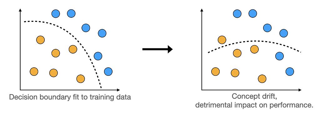
As a result, the model in production is being fed with differently distributed data compared to the ones it has seen during training. What are the consequences for its performance? Consider the following graphics.

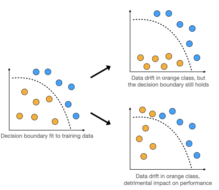
When the distribution of input data shifts too much, it may cross the model’s decision boundary resulting in worse performance.

Monitoring model performance

It is crucial to have proper monitoring in place to be able to detect early signs of slumping model performance. If we get alerted early enough, there might still be time to investigate its causes and decide to retrain the model, for instance.

In many cases, performance monitoring is a relatively standard task. It is the easiest when ground truth targets are available. Think about churn prediction. We have our model’s prediction for a group of users, and we know whether they have churned or not within a given timeframe. This allows us to calculate the metrics of our choice, such as accuracy, precision, or ROC AUC, and we can keep computing them constantly with new batches of data.

In other scenarios, we might not observe the ground truth targets directly, but still, receive some feedback on model quality. Think about spam filters. In the end, you will never know whether each particular email in your database is spam or not. But you should be able to observe some user actions that indicate it, such as moving messages from inbox to spam or taking an email classified as spam out of the spam folder. If the frequency of such actions does not increase, it may lead us to conclude that the model performance is stable.

Performance monitoring is easy, as long as ground truth targets or other direct feedback on model quality are available.

Finally, let’s consider the ultimate scenario in which little to no feedback on model quality is available. I was once part of a project working on the geolocation of mobile devices with the goal of predicting the user’s location in order to provide them with relevant marketing offers. While the entire business’ performance was indicative of the machine learning models’ quality, there were no ground truth data points available for each input the models received in production. How do we go about the monitoring then?

We can estimate model performance without ground truth labels when the model is properly calibrated.

Estimating model performance in the absence of ground truth data is tricky, but possible to accomplish. We just need one thing: a calibrated model. Let’s talk about what it means now.

Probability calibration

To understand probability calibration, let’s talk about probability itself first. Next, we will look at how the concept relates to classification models.

What is probability?

Surprisingly, there is no consensus as to what probability really is. We all agree it is a certainty measure and is typically expressed as a number between zero and one, with higher values denoting more certainty. And here the agreement ends.

There are two schools of thought about probability: frequentist (also known as classical) and Bayesian. A frequentist will tell you that “an event’s probability is the limit of its relative frequency in many trials”. If you tossed a coin many times, approximately half of the tosses will come up heads. The more tosses, the closer this rate is to 0.5. Therefore, the probability of tossing heads with a coin is 0.5.

A Bayesian would disagree, claiming that you can come up with probabilities without observing something happening many times, too. You can read more about the Bayesian way of thinking here and here. Let’s skip this discussion, however, since our main topic pertains to the frequentist definition of probability. Indeed, we need our classification model to produce frequentist probabilities.

Machine learning models & probability

Models that do produce frequentist probabilities are referred to as well-calibrated. In such a case, if the model returns an 0.9 probability of the positive class for a number of test cases, we can expect 90% of them to truly be the positive class.

Models that produce frequentist probabilities are referred to as well-calibrated.

Most binary classifiers, however, produce scores that tend to be interpreted as probabilities which they, in fact, are not. These scores are good for ranking — a higher number indeed means a higher likelihood of the positive class— but they are not probabilities. The reasons for this are specific to different model architectures, but in general, many classifiers tend to overpredict low probabilities and underpredict high ones.

Calibrating classifiers

One of the exemptions from the above rule is logistic regression. By construction, it models probabilities and produces calibrated results. This is why one way to calibrate an ill-calibrated model is to pass its predictions to a logistic regression classifier which should shift them appropriately.

Knowing all this, with our well-calibrated model at hand, we can finally turn to performance estimation without the targets!

Confidence-Based Performance Estimation

The algorithm that allows us to estimate model performance in the absence of ground truth, developed by NannyML, an open-source library for post-deployment data science, is called Confidence-Based Performance Estimation, or CBPE.

The idea behind it is to estimate the elements of the confusion matrix based on the expected error rates, which we know assuming the model is well-calibrated. Having the confusion matrix, we can then estimate any performance metric we choose. Let’s see how it works.

CBPE algorithm

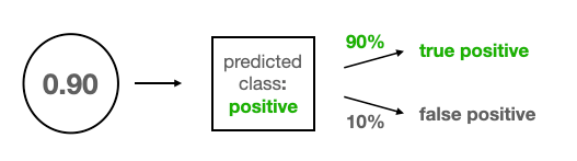
In order to understand the CBPE algorithm, let’s go through a simple example. Let’s say our model was used in production on three occasions and produced the following probabilities: [0.90, 0.63, 0.21]. And, of course, we don’t know the true target classes.

Consider the first prediction of 0.9, represented as a bubble on the picture below. Since it is larger than a typical threshold of 0.5, this example gets classified as a positive class. Hence, there are two options: if the model is right, it’s a true positive and if it’s wrong, it’s a false positive. Since the 0.9 produced by the model is a calibrated probability, we can expect the model to be right in 90% of similar cases, or to put it differently, we expect a 90% chance that the model is right. This leaves a 10% chance that the prediction is a false positive.

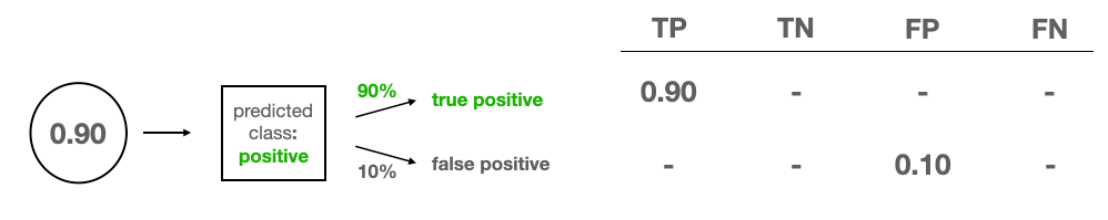
And so, we set up our confusion matrix. It has four entries: true positives (TP), true negatives (TN), false positives (FP), and false negatives (FN). As discussed, our first example has only two possibilities, which we distribute according to their probabilities.

Normally, a confusion matrix contains the counts of each prediction type, but the CBPE algorithm treats them as continuous quantities. And so we assign a 0.9 fraction of a true positive and a 0.1 fraction of a false positive to the matrix.

Enters the second test example for which the model outputs 0.63. Let’s put it in the picture as a new bubble below the first one. Again, it’s a TP or FP, so we assign the fractions accordingly.

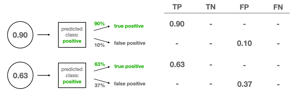
Finally, we have our third test case for which the prediction of 0.21 converts to a negative class. Let’s put it below the first two. This third example can either be a true negative with 100–21=79% probability, or a false negative with a 21% probability. We assign the corresponding fractions to our confusion matrix and sum the numbers for each of the four prediction types.

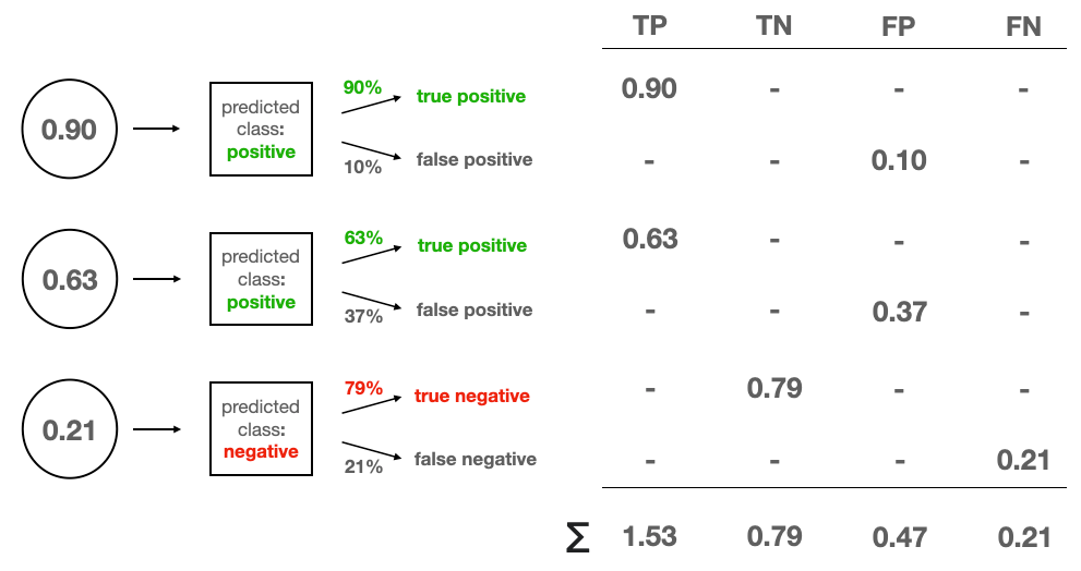
Once this is done, we can calculate any performance metric we desire. For instance, we can compute the expected accuracy by dividing the sum of TPs and TNs by the number of test cases: (1.53 + 0.79) / 3 = 0.77.

In a similar fashion, one might go about calculating precision, recall, or even the area under the ROC curve.

Danger zone: assumptions

There are no free lunches in statistics. Similar to most statistical algorithms, the CBPE does come with some assumptions that need to hold for the performance estimation to be reliable.

First, as we have already discussed, the CBPE assumes the model is calibrated. And, as we’ve said, most models are not by default. We can calibrate our model, e.g. by adding a logistic regression classifier on top of it, but this can potentially have a detrimental impact on accuracy metrics. Indeed, better calibration does not guarantee better performance — just a more predictable one. In situations where each accuracy percentage point is mission-critical, one might not be willing to sacrifice it.

Better calibration does not guarantee better performance — just a more predictable one.

Second, the CBPE algorithm works as long as there is no concept drift. Concept drift is the data drift’s even-more-evil twin. It’s a change in the relationship between the input features and the target.

CBPE only works in the absence of concept drift.

When it occurs, the decision boundary learned by the model is no longer applicable to the brave new world.

If that happens, the features-target mapping learned by the model gets obsolete and the calibration does not matter anymore — the model is simply wrong. Watch out for the concept drift!

CBPE with NannyML

NannyML, the company behind the CBPE algorithm, also provides its open-source implementation as part of their pip-installablenannyml Python package. You can check out the mathematically meticulous description of the algorithm in their documentation.

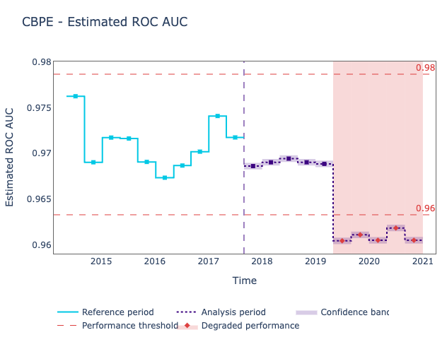
Estimating the ROC AUC of a classifier without knowing the targets takes literally five lines of code with nannyML, and produces good-looking visualization along the way, like the one below.

Do check out their Quick Start Guide to see how to implement it easily yourself!

Thanks for reading!

If you liked this post, why don’t you subscribe for email updates on my new articles? And by becoming a Medium member, you can support my writing and get unlimited access to all stories by other authors and myself.

Need consulting? You can ask me anything or book me for a 1:1 here.

You can also try one of my other articles. Can’t choose? Pick one of these:

• Don’t let your model’s quality drift away
• On the Importance of Bayesian Thinking in Everyday Life
• Calibrating classifiers

---

Estimating Model Performance without Ground Truth was originally published in Towards AI on Medium, where people are continuing the conversation by highlighting and responding to this story.

Join thousands of data leaders on the AI newsletter. It’s free, we don’t spam, and we never share your email address. Keep up to date with the latest work in AI. From research to projects and ideas. If you are building an AI startup, an AI-related product, or a service, we invite you to consider becoming a sponsor.

Published via Towards AI