Essentials of Pandas
Last Updated on July 25, 2023 by Editorial Team
Author(s): Adeel
Originally published on Towards AI.
All you need to know about the Pandas Library
Pandas is a data manipulation and analysis library that is built on top of NumPy. It is open-source and has easy-to-use data structures. Pandas is much like SQL and provides essential statistical and graphical support. In industry, many people use it as an alternative to excel as it provides basic data manipulation options.
To install pandas, the easiest way is to install Anaconda distribution. Anaconda contains different additional packages of python. Anaconda is also freely available. Check out the link for the installation of Anaconda.
To understand Pandas, the most important thing is to understand the data model and the two core data structures that the Pandas library supports. Series and DataFrame are the most common data structures that pandas support and are used to munge with tabular data.
Series is a 1D dimensional data structure, and DataFrame is a 2D dimensional data structure. You can compare a single column with the Series data structure and a sheet with rows and columns with the DataFrame data structure. In essence, a DataFrame can have a collection of a Series of objects.
The dataset that I am going to use is from one of our research projects. The dataset is for landslide prediction in Muzaffarabad, Pakistan, and it is freely available on Kaggle.
So, let’s jump in and get our hands dirty with Pandas.
.read_csv
import pandas as pd
df = pd.read_csv("landslide.csv")
df.head()

The above code imports pandas to read the dataset file and show the top five rows of the dataset. All the columns are ranged into different numbers. These numbers indicate the significance of each data point for the prediction of landslides.
The output shows a DataFrame that has several Series as columns like Aspect and Curvature. The Series is one-dimensional; therefore, it has a single axis.
.head
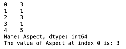
In the below code, I have printed the column Aspect from the dataset. In the below output, the left values indicate the index, and the right values indicate the actual value of the Aspect column. The .head method is used to print the top five rows of the dataset.
Aspect = df['Aspect']
print(type(Aspect))
print(Aspect.head())

.count and .size
To get the number of elements in the python series, we can use the .count method or the .size. The difference between .count method and .size is that the .count method excludes the NaN values while the .size counts them as well.
print(Aspect.count())
print(Aspect.size)

In the above example, Aspect does not have any missing values; therefore, the count and size method returns the same result.
.dtypes
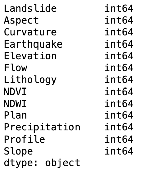
We can have multiple types of values, including categorical and Boolean values. The .dtype method is used to print the types of each column and the DataFrame.
print(df.dtypes)

.corr
The most important part of data manipulation is the aggregation method. These methods transfer the technical details into business prospects. The aggregation methods are corr, count, dtype, sum, unique, and std.
In the below example, the .corr method returns the Pearson Correlation. Pearson Correlation is a measure of the linear relationship between two variables, and it ranges from -1 to 1. Where — 1 or 1 indicates a strong relationship, while values close to 0 indicate a weak relationship.
print(df.corr())

.loc and .iloc
For pulling the data, we use indexing operators in Pandas. The .loc and .iloc are used for that purpose. The .loc is used to select data by label, while .iloc is used to select data by position.
print(Aspect.head())
print("The value of Aspect at index 0 is:", Aspect.iloc[0])

.plot
To understand the data in a better way, let's combine the capabilities of Pandas with a data visualization library Matplotlib. Pandas have native integration with Matplotlib. The Series object has the .plot attribute. This attribute can be used to create different plots.
Let’s use the %matplotlib inline to display the plots in the browser.
Aspect.plot.hist()

The plot histogram explains the skewness of data. It explains that we have more values of 3 than other values. To view the distribution of data, we can use a Box plot.
df['Earthquake'].plot.box()

There are several other plots that you can use depending upon need. Other plots include the line plot, series pie plot and bar plot.
.iteritems
Another data structure that was introduced earlier is the DataFrame. The DataFrame is Two-Dimensional, and it is used for analytical purposes. Now, let's move toward the DataFrame and print the unique values of each of the columns. In the below example, the .iteritems method is used to iterate over all the columns of a DataFrame.
for (columnName, columnData) in df.iteritems():
 print (columnName)
 print (set(columnData))

.describe
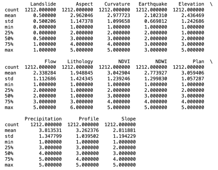
The Landslide variable, in this case, is the dependent variable, and all other are the independent variables. The values of each of the variables are normalized from 1 to 5, except Earthquake and Lithology.
The most common method used initially to explain the DataFrame is .describe method. The .describe method provides summary statistics of the numerical data.
df.describe()

So, that was it. I hope you learned something valuable from this blog. Please follow me on medium to read more about Data Science.
Until next time, Happy Coding…
Join thousands of data leaders on the AI newsletter. Join over 80,000 subscribers and keep up to date with the latest developments in AI. From research to projects and ideas. If you are building an AI startup, an AI-related product, or a service, we invite you to consider becoming a sponsor.
Published via Towards AI
Towards AI Academy
We Build Enterprise-Grade AI. We'll Teach You to Master It Too.
15 engineers. 100,000+ students. Towards AI Academy teaches what actually survives production.
Start free — no commitment:
→ 6-Day Agentic AI Engineering Email Guide — one practical lesson per day
→ Agents Architecture Cheatsheet — 3 years of architecture decisions in 6 pages
Our courses:
→ AI Engineering Certification — 90+ lessons from project selection to deployed product. The most comprehensive practical LLM course out there.
→ Agent Engineering Course — Hands on with production agent architectures, memory, routing, and eval frameworks — built from real enterprise engagements.
→ AI for Work — Understand, evaluate, and apply AI for complex work tasks.
Note: Article content contains the views of the contributing authors and not Towards AI.


