easy-explain: Explainable AI for images

Author(s): Stavros Theocharis

Originally published on Towards AI.

A quick and easy-to-use package for fast explainability results on images

Introduction

Understanding how artificial intelligence (AI) decides what to do is becoming increasingly important as AI finds more and more uses in everyday life. Particularly relevant here are image classification models, which employ AI to detect and label specific features in pictures, such as faces and objects. We need to be able to explain how these models come up with their predictions to make sure we can trust and account for them.

Explainable AI (XAI) is a collection of methods and techniques for making AI easier to understand and explain. Image classification techniques typically employ convoluted neural networks, making XAI all the more crucial. We may learn about the decision-making processes of these models, the attributes they use to recognize things, and any inherent biases they may have by employing XAI methods.

GitHub is teeming with new packages and repositories containing XAI methods derived from the literature or developed under custom cases.

In this article, I will present the “easy-explain” library, which comes from the new repository I created for explaining AI PyTorch models trained for images. I split this article into two sections. If you want to know how the easy-explain package works in detail, please read the first section, “easy-explain package in detail”. Otherwise, if you just want to know how to use the easy-explain package, please read directly “Simple use of the “easy-explain package”. For more information and guides, please have a look in the examples folder with the corresponding Jupyter notebooks.

For all the parts that will be shown below, we can consider as an example, the pre-trained Resnet50 model. We will load it from Torchvision:

import torchvision
model = torchvision.models.resnet50(pretrained=True).eval()

The images that are being used in the whole article are coming from Unsplash.

easy-explain package in detail

easy-explain uses under the hood Captum. Captum aids in comprehending how the data properties impact the model predictions or neuron activations, offering insights into how the model performs. Captum comes together with the Pytorch library. Currently, easy-explain is working only for images and only for Pytorch.

Captum allows for the unified application of several different cutting-edge feature attribution techniques, such as Guided GradCam and Integrated Gradients. In addition, the Occlusion methodology is being used.

Loading & Pre-processing of an image

Let’s get an image from Unsplash right away…

… and convert it into the desired format for our model with the needed transformations:

import requests
from PIL import Image
from io import BytesIO

response = requests.get("https://unsplash.com/photos/ZxNKxnR32Ng/download?ixid=MnwxMjA3fDB8MXxzZWFyY2h8NHx8bGlvbnxlbnwwfHx8fDE2NzU3OTY5NjE&force=true")
image = Image.open(BytesIO(response.content))

from torchvision import transforms

def process_image(image):
 center_crop = transforms.Compose([
 transforms.Resize(256),
 transforms.CenterCrop(224),
 ])
 normalize = transforms.Compose([
 # convert the image to a tensor with values between 0 and 1
 transforms.ToTensor(), 
 # normalize to follow 0-centered imagenet pixel rgb distribution 
 transforms.Normalize( 
 mean=[0.485, 0.456, 0.406],
 std=[0.229, 0.224, 0.225]
 )
 ])
 return normalize(center_crop(image)).unsqueeze(0)
input_img = process_image(image)

Get predictions

We can also get the pre-trained classes’ labels from the above Resnet50 model by clicking here. This is a JSON file, and we can load it directly from our save path:

import json

def load_data_labels(path: str = 'imagenet_class_index.json'):
 # Opening JSON file
 f = open(path)
 # returns JSON object as 
 # a dictionary
 data = json.load(f)
return data

labels = load_data_labels()

In order to provide an explanation for our findings, we must first determine the classes that require an explanation. This occurs as a result of the need to have one explanation at a time for each individual class.

So we need first to predict the needed classes.

In this walkthrough, we will focus on explaining the first option. In principle, a person is free to define and describe her own class on her own terms. But keep in mind that the first classes have meaning that needs to be explained. For example, if we have an image of a dog, we do not want to know why the model predicted that maybe our image represents a shark for a percentage of 0.005%.

So, as you probably guessed, we also get the needed percentages with the function below…

import torch

def predict_classes(input_img, labels, model, total_preds:int=5):
 # Find the score in terms of percentage by using torch.nn.functional.softmax function
 # which normalizes the output to range [0,1] and multiplying by 100
 out = model(input_img)
 percentage = torch.nn.functional.softmax(out, dim=1)[0] * 100
 # Find the index (tensor) corresponding to the maximum score in the out tensor.
 # Torch.max function can be used to find the information
 _, indices = torch.sort(out, descending=True)
 prediction = [(idx.item(), labels[str(idx.item())][1], percentage[idx].item()) for idx in indices[0][:total_preds]]
 
 return prediction
prediction = predict_classes(input_img, labels, model, 5)

Let’s see more of the XAI part, so…

How does Occlusion work?

Attribution can be calculated using a perturbation-based method by first replacing all adjacent rectangular regions with a particular baseline or reference and then calculating the change in output. Features spread over many hyperrectangles have their attributions calculated by averaging the differences in output from each hyperrectangle.

The initial patch is applied such that its corner is aligned with all zeros in the index range, and subsequent patches are applied in steps until the full dimension range has been patched. Keep in mind that this might lead to the final patch applied in a direction being smaller than the intended occlusion form due to being cut off.

Let’s dive into the code…

We need to import the needed functions:

import numpy as np
from captum.attr import visualization as viz
from captum.attr import Occlusion

Now we need the main functionality of Occlusion. As a target, we use the class we want to have the explanation for (as stated above).

Maybe we want to check the second or third in-the-row prediction. Keep in mind again that each time we can explain only one of the categories.

The important parts here are the following:

– strides: For each iteration, this specifies how far the occlusion hyperrectangle should be adjusted in each direction. This may be a single integer that is used as the step size in each direction for a single tensor input, or it can be a tuple of numbers that corresponds to the number of dimensions in the occlusion form.

– baselines: They define reference value which replaces each feature when occluded

– sliding_window_shapes: Shape of the patch (hyperrectangle) to occlude each input.

For more information, please read Captum’s Occlusion Docs.

def create_attribution(target, model, input_img):
 occlusion = Occlusion(model)
 strides = (3, 9, 9) # smaller = more fine-grained attribution but slower
 sliding_window_shapes=(3,45, 45) # choose size enough to change object appearance
 baselines = 0 # values to occlude the image with. 0 corresponds to gray
 attribution = occlusion.attribute(input_img,
 strides = strides,
 target=target,
 sliding_window_shapes=sliding_window_shapes,
 baselines=baselines)
 
 trans_attribution = np.transpose(attribution.squeeze().cpu().detach().numpy(), (1,2,0))

 return trans_attribution

And also some helpful functions:

def get_prediction_name_from_predictions(predictions):
''' A simple function to get the prediction name (we need it only for the title of the plots)'''
 name_of_prediction = predictions[0][1]
 name_of_prediction = name_of_prediction.capitalize().replace('_', ' ')
 return name_of_prediction

def get_image_titles(vis_types, vis_signs, name_of_prediction):
'''A helpful function to construct the titles of our images'''
 image_titles_list = []
 for i in range(len(vis_types)):

 if vis_signs[i]!="all":
 title = vis_types[i].capitalize().replace('_', ' ') + " for " + name_of_prediction
 else:
 title = vis_signs[i].capitalize().replace('_', ' ') + " " + vis_types[i].capitalize().replace('_', ' ') + " for " + name_of_prediction
 image_titles_list.append(title)
 return image_titles_list

Our below function will visualize the results. There are several combinations for vis_types and vis_signs. You can play a bit with them.

def create_explanation(attribution, image, name_of_prediction, vis_types=[["blended_heat_map", "original_image"]], vis_signs = [["all", "all"]]):
 center_crop = transforms.Compose([
 transforms.Resize(256),
 transforms.CenterCrop(224),
 ])
 image_titles_list = get_image_titles(vis_types, vis_signs, name_of_prediction)
 _ = viz.visualize_image_attr_multiple(attribution,
 np.array(center_crop(image)),
 vis_types,
 vis_signs,
 image_titles_list,
 show_colorbar = True
 )

Run the above functions:

prediction_name = get_prediction_name_from_predictions(prediction)
trans_attribution = create_attribution(prediction[0][0], model, input_img)

The main 5 predictions are:

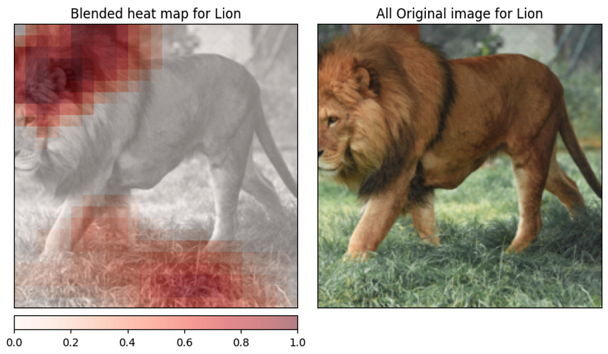
The model is pretty sure about the lion class. Let’s see the explanations…

(We will use separate parts for each explanation, each time only one set, e.g., “blended_heat_map”, “original_image”).

vis_types=[["blended_heat_map", "original_image"]]
vis_signs = [["positive","all"]]
number_of_sets = len(vis_types)

for i in range(number_of_sets):
 create_explanation(trans_attribution, image, prediction_name, vis_types = vis_types[i], vis_signs=vis_signs[i])

vis_types=[["blended_heat_map", "original_image"]]
vis_signs = [["negative","all"]]
number_of_sets = len(vis_types)

for i in range(number_of_sets):
 create_explanation(trans_attribution, image, prediction_name, vis_types = vis_types[i], vis_signs=vis_signs[i])

vis_types=[["masked_image", "original_image"]]
vis_signs = [["positive","all"]]
number_of_sets = len(vis_types)

for i in range(number_of_sets):
 create_explanation(trans_attribution, image, prediction_name, vis_types = vis_types[i], vis_signs=vis_signs[i])

vis_types=[["alpha_scaling", "original_image"]]
vis_signs = [["positive","all"]]
number_of_sets = len(vis_types)

for i in range(number_of_sets):
 create_explanation(trans_attribution, image, prediction_name, vis_types = vis_types[i], vis_signs=vis_signs[i])

By looking at the visualizations that are located above, we are able to comprehend some of the primary components that our model “saw” before concluding that the picture contains a lion. The legs, the mouth, and the belly are some of these parts.

The upper part of the lion’s head and the ground were the parts of our model that were able to convince it otherwise.

The ground should not play a major role in the selection since it should not help with the classification of the image. This is based on the training set and inserts some bias into our model.

So, let’s have one more try. This time, we will use the next predicted class:

input_img = process_image(image)
prediction = predict_classes(input_img, labels, model, 5)
prediction = prediction[1:]
prediction_name = get_prediction_name_from_predictions(prediction)
trans_attribution = create_attribution(prediction[0][0], model, input_img)

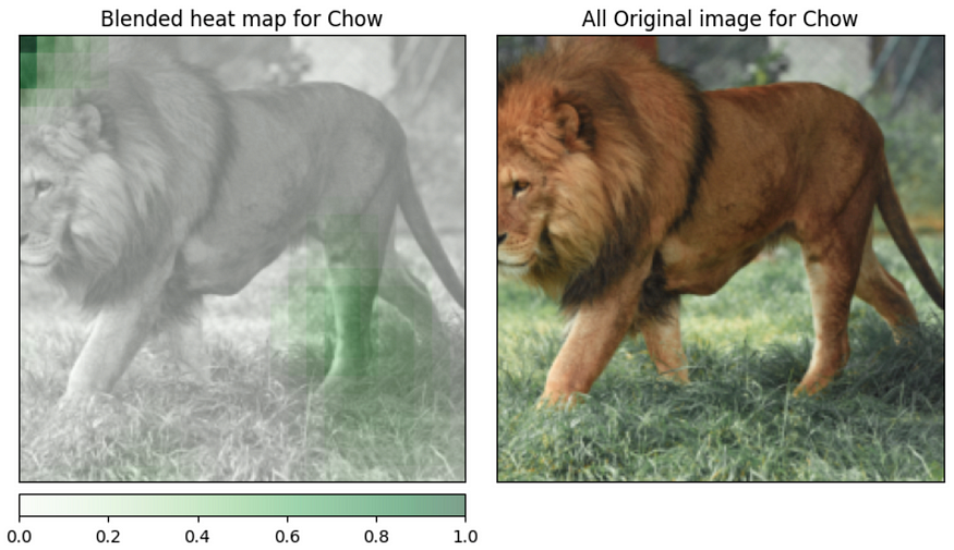
The prediction now becomes:

vis_types=[["blended_heat_map", "original_image"]]
vis_signs = [["positive","all"]]

number_of_sets = len(vis_types)

for i in range(number_of_sets):
 create_explanation(trans_attribution, image, prediction_name, vis_types = vis_types[i], vis_signs=vis_signs[i])

vis_types=[["blended_heat_map", "original_image"]]
vis_signs = [["negative","all"]]
number_of_sets = len(vis_types)

for i in range(number_of_sets):
 create_explanation(trans_attribution, image, prediction_name, vis_types = vis_types[i], vis_signs=vis_signs[i])

The animal’s legs primarily led the model to believe that the image represented chow with 0.40% of certainty.

Simple use of the “easy-explain package”

For the simple use of the package, just run the below lines of code:

(I have changed the link of the given image to show a variation in the results.)

from easy_explain.easy_explain import run_easy_explain

vis_types=[["blended_heat_map", "original_image"], ["blended_heat_map", "original_image"], ["masked_image", "original_image"], ["alpha_scaling", "original_image"]]
vis_signs = [["positive","all"], ["negative","all"], ["positive","all"], ["positive","all"]]

run_easy_explain(model, image_url = "https://unsplash.com/photos/aGQMKvPiBN4/download?ixid=MnwxMjA3fDB8MXxzZWFyY2h8M3x8c3F1aXJyZWwlMjBtb25rZXl8ZW58MHx8fHwxNjc1NzczNTIy&force=true", total_preds = 5, vis_types = vis_types, vis_signs = vis_signs, labels_path="imagenet_class_index.json")

And the results:

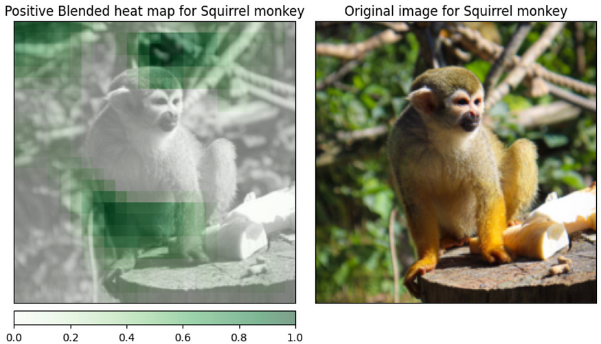
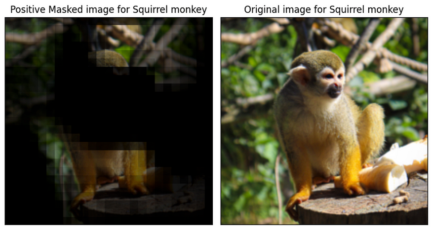
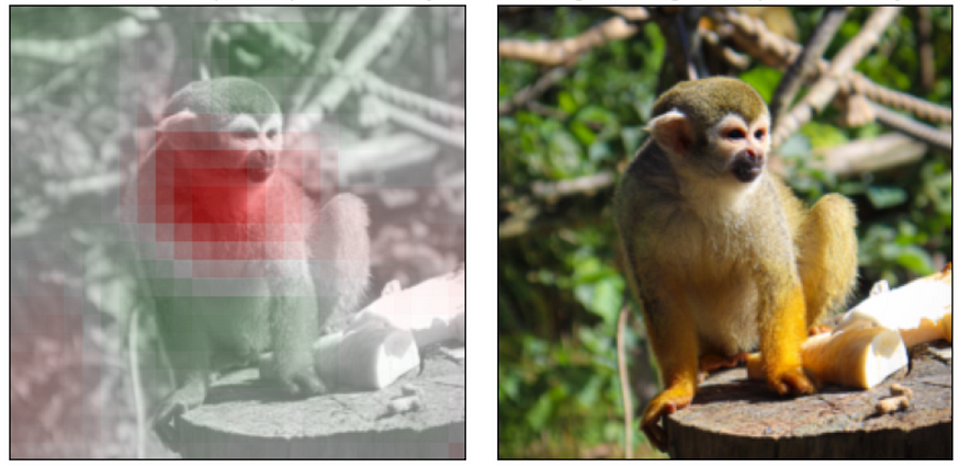
The great aspect of this case is that we have nice results that are easy to explain with only a few lines of code. The rapid construction and testing of the outputs of our models may be accomplished using this extremely easy and quick procedure.

Conclusion

In general, exploratory artificial intelligence (XAI) is an essential field that is helping to guarantee that artificial intelligence is trustworthy, interpretable, and transparent. By applying XAI methods to the development of image classification models, we are able to gain a better understanding of their operation and make well-informed choices on how they should be utilized.

In this article, I showcased the easy-explain package. Through it, someone can easily and quickly explain and check the predictions of the trained models.

If you liked this one and you also want to contribute, please check the contribution guide.

Join thousands of data leaders on the AI newsletter. Join over 80,000 subscribers and keep up to date with the latest developments in AI. From research to projects and ideas. If you are building an AI startup, an AI-related product, or a service, we invite you to consider becoming a sponsor.

Published via Towards AI