A Gentle Introduction to Automatic Differentiation
Last Updated on July 25, 2023 by Editorial Team
Author(s): Pablo Monteagudo Lago
Originally published on Towards AI.
As a student of Mathematics and Computer Science, it was natural for me to get interested in Artificial Intelligence, being this a field placed in the intersection of both of these knowledge areas: it sits on top of beautiful mathematical foundations while posing numerous computing challenges. Besides, its applications are uncountable, and it is expected to transform every industry from the ground up. In particular, Machine Learning, a major field of AI focused on building programs that learn to perform a task by extracting insights from data, has experienced remarkable growth in interest, both among researchers and practitioners.

But what does it mean for a machine to learn? Diving into the fundamentals of almost all machine learning algorithms, it can be seen that “learning” is formulated as the optimization of an objective function that measures how well the algorithm performs the task at hand. When it comes to the optimization of this function, it is frequent to rely on gradient-based optimization methods, which require the computation of the derivative of the objective function with respect to the model parameters.

However, when building, for instance, a neural network in TensorFlow or PyTorch, the actual computation of these derivatives is done transparently to the programmer using automatic differentiation. In this article, we discuss how this technique differs from other methods for computing derivatives, as well as provide a gentle introduction to how it works.
This article is intended to be the first in a series of articles on specific topics in Artificial Intelligence, hiding beautiful pieces of Mathematics which are often overlooked.
How to compute derivatives?
In the context of Machine Learning, we usually find ourselves working with a scalar function that measures the error in the predictions of our model over some sample data. For this function, we want to compute its gradient, that is, the vector of its partial derivatives with respect to the model parameters. Firstly, recall the definition of partial derivative:

Therefore, we want to compute the following vector:

Following, we illustrate the problems that automatic differentiation addresses by introducing the limitations of other differentiation techniques.
Manual differentiation
It consists of manually calculating the derivative. Then, the expression obtained is plugged into the program. This may be interesting from a theoretical viewpoint, but when we just need its numerical evaluations, it might be unnecessary as it is a time-consuming process and prone to error.

Symbolic differentiation
The differentiation of a function is a mechanistic process and, therefore, can be carried out by a computer program (e.g., Mathematica, Maple…).

However, the result may end up being a large expression whose evaluation cannot be done efficiently. This problem is referred to as expression swell.
To illustrate this, consider the following example:

The symbolic form of its gradient is shown below:

Besides, symbolic differentiation is only applicable to functions that take a closed-form. However, if the function is expressed as a computer program with loops, recursion… this may not be possible to determine:
def f(a: float, b: float) -> float:
 c : float = 0.0
 if a > b:
 for i in range(10):
 c += a*i
 else:
 c = a*b
 return c
Numerical differentiation
Recall that the partial derivatives of a function are formally defined as a limit. Therefore, taking a sufficiently small value for h we can approximate its value by the difference quotient:

However, this approximation is numerically unstable (we are dividing by a number close to zero and subtracting numbers that may be approximately equal).
Besides, in case we are computing the full gradient, this technique would require n+1 evaluations of the objective function, which may be prohibitively expensive.
Automatic Differentiation
Automatic differentiation addresses the issues of the techniques above. This technique comes from the observation that every numerical algorithm ultimately narrows down to the evaluation of a finite set of elementary operations with known derivatives.
For example, consider the function:

Following the observation above, we can adopt two equivalent notations for representing any numerical algorithm:
- Evaluation Trace or Wengert list. The function is constructed using intermediate variables vᵢ and elementary operators. In the example below, we use the three-part notation by Griewank and Walther.

- Computational Graph. The value of each variable is determined by applying a specific elementary operator over some set of input variables. As a result, there exists a relation of precedence among variables, which we represent as the edges of a Directed Acyclic Graph. Its nodes are the variables involved in the computation of the function.

Note that we colored in blue the input variables, in green the intermediate variables, and in yellow the output variables.
Both of these representations allow us to keep all the expressivity of a program with non-linear control flow because we can linearize the trace of execution. Besides, for computing derivatives, we only need to take into account the numerical evaluations during the execution of the program, along with their order, regardless of the control flow path. As a consequence, automatic differentiation allows us to differentiate functions with a non-closed-form.
To illustrate how the evaluation trace comes up naturally when executing a numerical algorithm, let’s spice up this article with some code. First, we’ll add a wrapper around the float type in Python, which we call Variable. This allows us to override its operators. Besides, a unique name is assigned to every variable.
We can override the operators for our Variable to keep track of the elementary operations performed during the evaluation of our function. Our multiplication operator is defined as follows:
Creating similar functions for the rest of the operators, we can compute our function f:
The execution of this code shows us the evaluation trace. Note that in the evaluation of our function, we are traveling the computational graph in the natural order according to the precedence relation. Therefore, this run is usually named forward pass.
v-1 = 2
v0 = 1
v1 = log(v-1) = 0.693
v2 = sin(v0) = 0.841
v3 = v-1 * v2 = 1.683
v4 = v1 + v3 = 2.376
This evaluation trace will be the basis for computing the gradient of our vector f. However, we need to store it, so we can replicate the elementary operations involved, along with the order in which they were carried out during the evaluation. Since our evaluation trace is a linear representation of the computation, it is natural to record it using a list, which, in this context, is commonly named tape. Its entries are defined as follows:
For each elementary operation, we record its inputs, outputs, and a closure, named propagate, which is the key component to computing the gradients of our function. Therefore, we have to extend our operators to ensure that each computation is recorded on the tape:
Reverse Mode Automatic Differentiation
Reverse Mode Automatic Differentiation can be thought of as a generalized backpropagation algorithm in the sense that derivatives are propagated backward from a given output. To do so, we complement each intermediate variable vᵢ with an adjoint:

These adjoints represent, in plain words, the contribution of each variable to the change in the output. Precisely, the adjoints assigned to the input variables are the partial derivatives we want to determine for our gradient.
The effective computation of these adjoints is carried out by traveling the graph from the output to its inputs. The underlying principle behind this is the application of the multivariate chain rule. For our example, we can use it to compute the partial derivative w.r.t. the first input variable:

In plain words, what the multivariate chain rule tells us is that, in order to compute each adjoint, we have to follow two rules:
- Multiply the partial derivatives along a path from the output variable to the chosen variable.
- Add up the results of the previous computation for all the paths.
However, we have two input variables, so it is desirable that we only have to travel the graph once for computing both partial derivatives, a requirement that would be paramount if we worked, for example, with hundreds or thousands of input variables. Precisely, the adjoints can be thought of as a book-keeping device for saving common subexpressions to ensure that each edge in the graph is traveled only once.

Therefore, for performing the backward pass, in which we compute the adjoints for each intermediate variable, we need to keep track of the partial derivatives for each intermediate variable w.r.t. its inputs. This is done by the closure we record in our tape. Let’s dive into the details of its implementation for the operator multiplication:
First, we compute the partial derivatives of the output, denoted as r, with respect to its inputs, e.g., the variables self and rhs:
The parameter dL_outputs corresponds to the adjoint of the output variable r. Note that, although it is formally defined as a List, we know in advance that it contains exactly one element, as this is the number of outputs for our operator. We can use this adjoint to update the adjoints of its input variables:
What we are doing is sticking to the first of the rules stated above by multiplying the partial derivatives along a path from the output to each of the input variables for the variable r.
Therefore, to compute the gradient for our function, we have to travel the graph backward, computing the adjoints for each intermediate variable by adding up the contributions that the closure propagate returns:
Let’s see how this function allows us to compute the gradient for the function defined before:
The execution of these cells returns the following output:
dv4 ------------------------
v6 = v5 * v2 = 0.841
v7 = v5 * v-1 = 2.000
v8 = cos(v0) = 0.540
v9 = v7 * v8 = 1.081
v10 = 1.0 / v-1 = 0.500
v11 = v5 * v10 = 0.500
v12 = v6 + v11 = 1.341
dv4_dv4 = v5
dv4_dv1 = v5
dv4_dv3 = v5
dv4_dv-1 = v12
dv4_dv2 = v7
dv4_dv0 = v9
------------------------
dx1 1.3414709848078965
dx2 1.0806046117362795
It works! This is precisely the result for the evaluation of the gradient for our function at (2,1).
Linear Regression with Gradient Descent
The previous example intended to be illustrative of how automatic differentiation works. However, it is convenient to demonstrate its potential in a more down-to-earth context.
In the following example, our objective is to predict the values for the dependent variable Y using the values for X. The relationship between these two random variables is modeled by the following relationship:

In our example, we set w₀=w₁=1. These values are supposed to be unknown and therefore, our objective is to infer them from the sample data or, in other words, fit a linear model to the sample data.
input_size = 50
X = np.random.random(input_size)
noise = np.random.normal(0, 0.05, input_size)
y_truth = X + 1 + noise

When fitting a linear model to our sample data, our objective is to minimize the differences between the predictions of the model and the ground truth over the sample data. In this example, the error is measured using the following loss function:

And how do we find the parameters that minimize this function? We will use gradient descent to optimize this function. That is, we will iteratively adjust the parameters using their gradients:

Therefore, we need to compute the gradient at each iteration. Although the differentiation of our loss function is simple, we rely on our little framework to do it for us:
We included a naive vectorization by defining the functions to_var and to_vals. This allows us to use numpy functions that help make the code more readable. Note that the computation is done using our well-known function grad. After running this code, we can visualize the line fitted to the sample data:

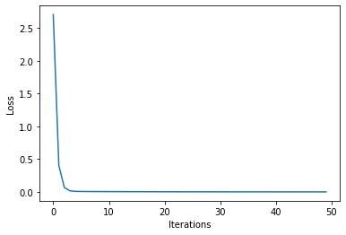
Besides, we can plot the loss values against the iterations:

Note that in the first iterations, the loss decreases very rapidly, converging to zero. Our framework for automatic differentiation works! We can also plot the trajectory of our gradient steps over the parameter space:

The illustration above shows how our parameters converge to the global minimum of our loss function in the point (1,1). However, the convergence is slow after some iterations, which should not come as a surprise since our learning rate is fixed during training.
In conclusion, we have developed a little framework that allows us to differentiate functions in several variables automatically. However, it is important to remark that it is a minimal working example and the algorithms provided by frameworks like TensorFlow and PyTorch are considerably more complex. The implementation is based on this Colab repository. To go into more detail, I would suggest checking it out.
The full code for this article can be found in my GitHub.
Bibliography
[1] A. Griewank and A. Walther. Evaluating derivatives: principles and techniques of algorithmic differentiation (2008). Society for industrial and applied mathematics.
[2] A. G. Baydin, B. A. Pearlmutter, A. A. Radul and J.M. Siskind. Automatic differentiation in machine learning: a survey (2018). Journal of Machine Learning Research, 18, 1–43.
Join thousands of data leaders on the AI newsletter. Join over 80,000 subscribers and keep up to date with the latest developments in AI. From research to projects and ideas. If you are building an AI startup, an AI-related product, or a service, we invite you to consider becoming a sponsor.
Published via Towards AI
Towards AI Academy
We Build Enterprise-Grade AI. We'll Teach You to Master It Too.
15 engineers. 100,000+ students. Towards AI Academy teaches what actually survives production.
Start free — no commitment:
→ 6-Day Agentic AI Engineering Email Guide — one practical lesson per day
→ Agents Architecture Cheatsheet — 3 years of architecture decisions in 6 pages
Our courses:
→ AI Engineering Certification — 90+ lessons from project selection to deployed product. The most comprehensive practical LLM course out there.
→ Agent Engineering Course — Hands on with production agent architectures, memory, routing, and eval frameworks — built from real enterprise engagements.
→ AI for Work — Understand, evaluate, and apply AI for complex work tasks.
Note: Article content contains the views of the contributing authors and not Towards AI.


