Customer Segmentation and Time Series Forecasting Based on Sales Data
Last Updated on October 20, 2024 by Editorial Team
Author(s): Naveen Malla
Originally published on Towards AI.
This is the third article in a 3-part series. In the first part, I covered initial exploratory data analysis steps and in the second, Customer Segmentation. You don’t have to read those before getting into this article, but they’ll give you some great insights and set you up for the more exciting stuff we’re about to cover.
Customer Segmentation and Time Series Forecasting Based on Sales Data #1/3
project that got me an ml internship
pub.towardsai.net
Customer Segmentation and Time Series Forecasting Based on Sales Data #2/3
project that got me a ml job
pub.towardsai.net
Put simply, time series forecasting is a technique used to predict future values based on historical data.
We have two options for training the forecasting model:
- Train one single model for all SKUs.
- Captures general trends and patterns in the data.
- Might not be able to capture the SKU specific patterns.
2. Train one model for each SKU.
- Captures SKU specific patterns.
- Might be computationally expensive.
💡 Let’s Revisit the Dataset
This is a typical sales dataset with different features, but since we are only interested in predicting the future sales, we can drop the rest of the columns and only keep the necessary ones.
df = pd.read_csv('data/sales.csv')
df = df.drop(['order_number', 'customer_number', 'type', 'month', 'category', 'revenue', 'customer_source', 'order_source'], axis=1)
df['order_date'] = pd.to_datetime(df['order_date'])
df['day'] = df['order_date'].dt.date
df.head()

In our case, I chose to consider the second option and build a model for each product.
df_ke0001 = df[df[‘item_number’] == ‘KE0001’]
df_ke0001 = df_ke0001.groupby(‘day’).agg({‘quantity’:’sum’}).reset_index()
df_ke0001.columns = [‘ds’, ‘y’]
print(df_ke0001.head(10))
print(df_ke0001.shape)
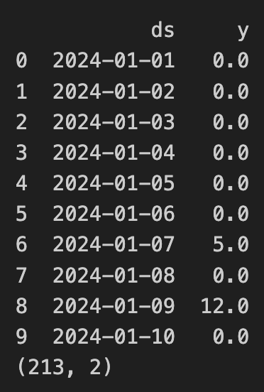
y is total quantity of the product KE0001 sold on given date. We can observe that the data is not continuous, the product is not bought every so we need to fill in the missing days with 0 sales.
from datetime import date, timedelta
start_date = date(2024, 1, 1)
end_date = date(2024, 7, 31)
delta = timedelta(days=1)
days = []
while start_date <= end_date:
 days.append(start_date)
 start_date += delta
df_ke0001 = df_ke0001.set_index('ds').reindex(days).reset_index()
df_ke0001['y'] = df_ke0001['y'].fillna(0)
df_ke0001.columns = ['ds', 'y']
print(df_ke0001.head(10))
print(df_ke0001.shape)

Plot the sales for KE0001
plt.figure(figsize=(15, 6))
plt.plot(df_ke0001[‘ds’], df_ke0001[‘y’])
plt.title(‘Daily sales of KE0001’)
plt.show()

🎯 Stationary or Non-Stationary Data?
Stationary data:
- The statistical properties of the data like mean do not change over time. Or at least not so much.
- Time series models usually work better with stationary data.
How to check if the data is stationary?
- We use the Augmented Dickey-Fuller test.
- This test checks if the properties of data like mean and standard deviaton are constant over time.
Augmented Dickey-Fuller test gives us two values.
1) p-value: If less than 0.05, the data is stationary.
2) ADF Statistic: The more negative this value, the stronger the evidence that the data is stationary.
from statsmodels.tsa.stattools import adfuller
result = adfuller(df_ke0001['y'])
print(f'ADF Statistic: {result[0]}')
print(f'p-value: {result[1]}')

- The ADF Statistic is far less than 0 and the p-value is far less than 0.05.
- Safe to say the data is stationary.
📉 Rolling Mean and Rolling Standard Deviation
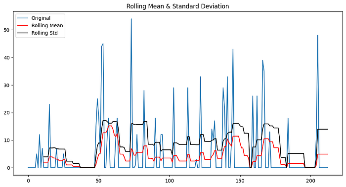
- Yet another way to make sure the data is stationary.
- These metrics calculate the mean and strandard deviation continuously over a window of time.
rolmean = df_ke0001[‘y’].rolling(window=12).mean()
rolstd = df_ke0001[‘y’].rolling(window=12).std()

plt.figure(figsize=(12, 6))
plt.plot(df_ke0001['y'], label='Original')
plt.plot(rolmean, color='red', label='Rolling Mean')
plt.plot(rolstd, color='black', label='Rolling Std')
plt.title('Rolling Mean & Standard Deviation')
plt.legend()
plt.show()

In our case…
- There are fluctuations in the data due to the high spikes in the sales.
- But the overall trend seems to be stationary. Not moving up or down.
📊 Different Models That Can Be Used for Time Series Forecasting
- ARIMA (AutoRegressive Integrated Moving Average):
Best for: Non-seasonal data without trends. - SARIMA (Seasonal ARIMA):
Best for: Seasonal data with patterns that repeat at regular intervals. - Prophet:
Best for: Handling seasonality, holidays, and missing data. - LSTM (Long Short Term Memory):
Best for: Complex data with long-term dependencies.
- Missing data is a key factor for us here because we have many days where there are no sales. So we choose Prophet.
- Analysis and Results with ARIMA in APPENDIX for further reading.
About Prophet
- Developed by Researchers at Facebook.
- Decomposes time series into trend, seasonality, and holidays.
- Handles missing data.
- Automatically detects change points in the time series.
Let’s train the model and make the data frame ready for accommodating sales for next 3 months.
# train the model
from prophet import Prophet
model = Prophet(interval_width=0.95)
model.add_seasonality(name='monthly', period=30.5, fourier_order=10)
model.fit(df_ke0001)

future_dates = model.make_future_dataframe(periods=90, freq='D')
future_dates.tail()

Get the forecast
forecast = model.predict(future_dates)
# Clip the forecasted values to be zero or above
forecast['yhat'] = forecast['yhat'].clip(lower=0)
forecast['yhat_lower'] = forecast['yhat_lower'].clip(lower=0)
forecast['yhat_upper'] = forecast['yhat_upper'].clip(lower=0)
forecast[['ds', 'yhat', 'yhat_lower', 'yhat_upper']].tail()

Here…
- yhat: Forecasted value for the target variable.
- yhat_lower: Lower bound of the forecast (clipped to 0 in this case).
- yhat_upper: Upper bound of the forecast, showing the highest possible value.
🔮 Analysing various trends in the data.
model.plot_components(forecast);

Understanding the y-axis:
- The y-axis in these plots represents the contribution of each component (trend, weekly seasonality, monthly seasonality) to the overall forecast.
- For example, a value of -2 on Monday indicates that Mondays typically see 2 units fewer than the baseline trend
Observations:
- Trend Plot: Reflects a slow and steady increase in the data over time, as indicated by the slight upward slope.
- Weekly Seasonality Plot: Shows how different days of the week affect the data, with some days (like Saturdays) showing higher activity than others (like Mondays).
- Monthly Seasonality Plot: Reveals specific days in the month that have significant impact on the sales, such as around the middle of the month.
📈 Time for the Forecast
# Ensure both are in datetime format
df_ke0001[‘ds’] = pd.to_datetime(df_ke0001[‘ds’])

# Filter out the historical period from the forecast
forecast_filtered = forecast[forecast['ds'] > df_ke0001['ds'].max()]
# Plot only future forecasts
plt.figure(figsize=(15, 6))
plt.plot(df_ke0001['ds'], df_ke0001['y'], label='Original Data')
plt.plot(forecast_filtered['ds'], forecast_filtered['yhat'], label='Forecast', linestyle=' - ')
plt.fill_between(forecast_filtered['ds'], forecast_filtered['yhat_lower'], forecast_filtered['yhat_upper'], color='blue', alpha=0.2, label='Uncertainty Interval')
plt.title('Comparison of Original Data and Future Forecast')
plt.legend()
plt.show()

Forecast Overview:
- The forcast captures the general trend and presence of spikes but doesn’t fully replicate the spike patterns because it might see them as irregular.
- Prophet model can efficiently capture seasonality and trends but might miss specific, irregular spikes.
🛠 How to make it better?
More accurate predictions could be achieved by adding information like promotions, holidays, or other significant events that might influence sales.
Now we forecast for all individual items in the dataset for the next 90 days.
- We get all the unique items.
- Then, iterate over to train, forecast and save the forcasted data for each item.
unique_items = df[‘item_number’].unique()
print(unique_items.shape)
print(unique_items[:5])
We basically build 1000 small models, each for a different item and get the individual forecasts.
import pandas as pd
from prophet import Prophet

# Create a new DataFrame to store the forecasted data
forecasted_data = pd.DataFrame(columns=['item_number', 'August', 'September', 'October'])
# Loop through all the unique items
for item in unique_items:
 df_item = df[df['item_number'] == item]
 df_item = df_item.groupby('day').agg({'quantity': 'sum'}).reset_index()
 df_item.columns = ['ds', 'y']

 # Fill in the missing days
 df_item = df_item.set_index('ds').reindex(days).reset_index()
 df_item['y'] = df_item['y'].fillna(0)

 # Train the model
 model = Prophet(interval_width=0.95)
 model.add_seasonality(name='monthly', period=30.5, fourier_order=10)
 model.fit(df_item)

 # Forecast the next 90 days
 future_dates = model.make_future_dataframe(periods=90, freq='D')
 forecast = model.predict(future_dates)
# Clip the forecasted values to be zero or above
 forecast['yhat'] = forecast['yhat'].clip(lower=0)
 forecast['yhat_lower'] = forecast['yhat_lower'].clip(lower=0)
 forecast['yhat_upper'] = forecast['yhat_upper'].clip(lower=0)

 # Save the forecasted data
 august_sum = forecast['yhat'].iloc[212:243].sum()
 september_sum = forecast['yhat'].iloc[243:273].sum()
 october_sum = forecast['yhat'].iloc[273:304].sum()

 # Create a DataFrame for the current item
 forecasted_item = pd.DataFrame({
 'item_number': [item],
 'August': [august_sum],
 'September': [september_sum],
 'October': [october_sum],
 'Total': [august_sum + september_sum + october_sum]
 })

 # Use pd.concat() to append the data
 forecasted_data = pd.concat([forecasted_data, forecasted_item], ignore_index=True)
# Display the forecasted data
print(forecasted_data.head(10))
# save the forecasted data in a csv file
forecasted_data.to_csv('data/forecasted_data.csv', index=False)
Get the top 100 products in the original data and forecasted data and see how many match.

Almost half of the top 100 products in the original data match with the forecasted data.
Next, let’s compare the total sales of the top 10 products in the original data and forecasted data.

Observation:
The predictions show an increase in sales in next three months, following the slight increase of trend in the original data as seen in the first part where we did EDA.
I also created two models trained on weekly sales and daily sales using ARIMA. I put that code and explanation in Appendix section of the notebook so as to not make this too long.


Star the repo for further/future reference here:
GitHub – naveen-malla/Customer-Segmentation-and-SKU-Forecasting: This repo contains code for…
This repo contains code for performing customer segmentation and sales forecast prediction on a company's sales data. …
github.com
If you found the post informative, please
- hold the clap button for a few seconds (it goes up to 50) and
- follow me for more updates.
It gives me the motivation to keep going and helps the story reach more people like you. I share stories every week about machine learning concepts and tutorials on interesting projects. See you next week. Happy learning!
Connect with me: LinkedIn, Medium, GitHub
Join thousands of data leaders on the AI newsletter. Join over 80,000 subscribers and keep up to date with the latest developments in AI. From research to projects and ideas. If you are building an AI startup, an AI-related product, or a service, we invite you to consider becoming a sponsor.
Published via Towards AI
Towards AI Academy
We Build Enterprise-Grade AI. We'll Teach You to Master It Too.
15 engineers. 100,000+ students. Towards AI Academy teaches what actually survives production.
Start free — no commitment:
→ 6-Day Agentic AI Engineering Email Guide — one practical lesson per day
→ Agents Architecture Cheatsheet — 3 years of architecture decisions in 6 pages
Our courses:
→ AI Engineering Certification — 90+ lessons from project selection to deployed product. The most comprehensive practical LLM course out there.
→ Agent Engineering Course — Hands on with production agent architectures, memory, routing, and eval frameworks — built from real enterprise engagements.
→ AI for Work — Understand, evaluate, and apply AI for complex work tasks.
Note: Article content contains the views of the contributing authors and not Towards AI.


