RMSprop Explained: a Dynamic learning rate
Last Updated on July 17, 2023 by Editorial Team
Author(s): Skander Menzli
Originally published on Towards AI.
Introduction:
Gradient descent is one of the most fundamental building blocks in all of the machine learning, it can be used to solve simple regression problems or build deep neural networks, hence there is a lot of value in trying to find ways to optimize it. In this article, we’ll look at one of the most relevant ones RMSprop, and explain it clearly.
Vanilla Gradient descent :
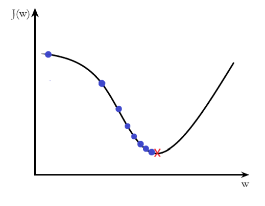
let’s recap regular old gradient descent; we got our cost function J(W), we calculated its gradient vector then we updated our parameters W by taking steps in the opposite direction to the gradient by subtracting it from the current weights, and we keep iterating until we reach the minimum

Pretty straightforward so how can we improve it, well the one hyperparameter that we can tune in equation (1) is the learning rate, the problem is taking it too small, and gradient descent will be very slow, take it too big and it will diverge.

Plus we’re using the same learning rate for all the weight parameters in the gradient vector, so it doesn’t take into account how much each weight is contributing to the loss, and this will cause gradient descent to oscillate a lot until it reaches the minimum.

So what we need is a dynamic learning rate for each weight
Optimization:
So how do we want our learning rate to change? The idea is for every weight, we want to take big steps when the curvature of the J(w) space is low because there is no risk of overshooting due to the gradient being large and small steps when the curvature is big (large gradient).

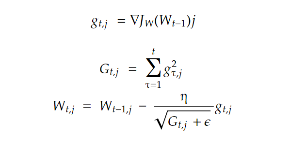
The curvature represents the rate of change of our cost function, and we can measure that by simply calculating the l2 norm of the gradient vector. Here is our new gradient descent (for one weight wj):

We accumulate the square of all past gradients in G, and then we take gradient descent steps with a scaling down of the gradient vector with a factor of sqrt(G +????) with ???? a smoothing term to avoid division by zero, usually equal to 10^-(10) and η is global learning. That’s how we get a dynamic learning rate that is inversely proportional to the magnitude (curvature), so big gradients have small learning rates and small gradients have large rates. This way, the progress over each dimension will even out over time, and that will help point the resulting updates more directly toward the minimum (fewer oscillations).

And that’s the adagrad( adaptive gradient) algorithm. But going by the title of this article, we are not done yet because adagrad has one problem, since we are scaling down by the sum of the magnitude of all past gradients after enough iteration, the learning rate gets scaled down so much that the algorithm stops completely before reaching the minimum.
RMSProp (Root mean squared propagation) fixes this by taking a running average of past gradients instead of a sum of all gradients since the beginning of training with the decay rate γ typically set to 0.9

Conclusion:
In conclusion, RMSProp is a very intuitive way to optimize gradient descent by dynamically changing the learning rate of each weight, and it’s usually used in combination with an other optimization technique, momentum, for better performance.
Join thousands of data leaders on the AI newsletter. Join over 80,000 subscribers and keep up to date with the latest developments in AI. From research to projects and ideas. If you are building an AI startup, an AI-related product, or a service, we invite you to consider becoming a sponsor.
Published via Towards AI
Towards AI Academy
We Build Enterprise-Grade AI. We'll Teach You to Master It Too.
15 engineers. 100,000+ students. Towards AI Academy teaches what actually survives production.
Start free — no commitment:
→ 6-Day Agentic AI Engineering Email Guide — one practical lesson per day
→ Agents Architecture Cheatsheet — 3 years of architecture decisions in 6 pages
Our courses:
→ AI Engineering Certification — 90+ lessons from project selection to deployed product. The most comprehensive practical LLM course out there.
→ Agent Engineering Course — Hands on with production agent architectures, memory, routing, and eval frameworks — built from real enterprise engagements.
→ AI for Work — Understand, evaluate, and apply AI for complex work tasks.
Note: Article content contains the views of the contributing authors and not Towards AI.


