You’re Missing The Point Behind PCA

Author(s): Nandini Tengli

Originally published on Towards AI the World’s Leading AI and Technology News and Media Company. If you are building an AI-related product or service, we invite you to consider becoming an AI sponsor. At Towards AI, we help scale AI and technology startups. Let us help you unleash your technology to the masses.

Just as with most things in computer science, understanding what PCA (Principal Component Analysis) is or why it works takes hours of digging and sifting through complicated documentation. When trying to learn about PCA, most resources that I came across glossed over how/why PCA actually worked and didn’t give me any intuition behind the algorithm’s motives.

My goal with this article is to compile an easy-to-understand account of what PCA actually is and why it works. I will provide links to resources for any further study.

Hello! I am Nandini Tengli, a college junior majoring in Computer Science. This is my CS blog, where I try to document what I learn in the most non-jargony way possible. If you are like me and love digging deep to get a good understanding of things but end up spending hours just trying to decrypt documentation, then you are in the right place.

Links to all resources are at the bottom of the article!

What you need to be familiar with before trying to understand the math behind PCA:

• Eigendecomposition
• Linear Transformation

If you’ve never heard of these terms, then you should probably take a look at the resources at the bottom before reading this. If you have even a vague familiarity with what these terms mean, then you can start reading this article and revisit these topics as you need to!

Principal Component Analysis

Despite PCA being commonly known as a dimensionality reduction technique, this is not entirely accurate.

If there is one thing you take away from this article, it should be this: PCA is just a Linear transformation — a change of perspective if you will — of the data. The idea is to get a better understanding of the underlying patterns in your data by changing the perspective through which you view your data.

But what exactly is a linear transformation?

Let us say your data is a big box of colored marbles, with each color in its own separate box. Viewing your data (marbles) like this helps you understand certain things, like the number of colors the marbles are available in. But what if there were other patterns in your marbles that you were missing simply because you chose to organize your marbles by color? Applying the PCA algorithm on this box would be like shaking the box up and reordering it by the size of the marbles instead of the colors. In doing so, different patterns (one that concerns size in this case) come to the forefront.

Of course, this is a simple analogy, and we should be careful not to extend its implications. The idea is to understand that PCA is a linear transformation technique — a change of perspective — of the data.

So all this algorithm really does is a cluster or order your data by a different feature/set of features (dimensions or axis — here, we changed the feature from color to size) in the hopes of getting a better understanding of the data and the trends in it.

The real use case of PCA actually lies in the way it constructs the transformation matrix — the way it picks the ‘features’ or the ‘dimensions’ to organize your data.

The way PCA actually comes up with this new set of dimensions is by maximizing for ‘spread’ or variance in the data. The intuition behind this is that: given our dataset has good measurements (minimal noise), we assume that the directions of largest variances capture the most interesting patterns/dynamics (signals) in our data. So changing our reference frame — our basis — — to align with the directions of the largest variances allows us to analyze better/study these patterns in our data.

Another goal while working with massive datasets is to minimize redundancy in the dataset. For instance: given two features that are extremely correlated, we can reduce redundancy by recording just one of the features instead of both of them. This is because we can always use the relationship between the two features to produce the data for the second one. Since PCA also has this goal of reducing redundancy also built into the algorithm.

PCA orders the new axes/dimensions/features from the most ‘useful’ to the least ‘useful’. This means that we can drop the less useful attributes easily and thus better optimize our learning algorithms. This ‘getting rid of attributes’ is what is referred to as projecting the data onto a lower dimensional subspace in linear algebra. Since these attributes are ‘new’ — completely different — from the original attributes of our data, we can reduce the dimensionality of the data without having to explicitly ‘delete’ any of the original attributes. Since we have the transformation matrix, we can always re-derive the original ordering of the data by using the inverse of this matrix. This will become more clear when we apply this algorithm to compress a large image of a dying star later on in the article. This is what makes PCA a popular choice for dimensionality reduction in data science.

‘Usefulness’ for the PCA algorithm is based on variance. It orders the dimensions — the principal components — by the amount of variance they capture. The first dimension — the first principal component — is going to be along the direction of the most varied data. The second principal component has to be orthogonal (perpendicular) to the first principal component and in the direction of the second highest variance. This is repeated to find the other principal components. We restrict each new principal component to being orthogonal to all the previous components since it allows us to take advantage of linear algebra.

There are a couple of avenues to perform PCA using python:

• Sklearn’s decomposition module. This is the most straightforward method to perform PCA
• From scratch: using the covariance matrix and eigendecomposition: the best way to understand the math behind the algo
• Singular Value Decomposition: another great Linear Algebra technique that allows us to skip a couple of steps!

We are going to explore the latter two since the first method is heavily explored and is straightforward.

The Algorithm:

• The first step is to center the data around the mean by subtracting the mean from the data. If your data set has attributes, each of which has widely different variances, but if the importance of attributes is independent of this variance, then you should divide each observation in the column by the standard deviation of that column’s attribute.
• The reason this is an important consideration is that we are maximizing the direction of variance. This means that one of the attributes of your data has a much bigger range than the others: for instance, if the salary attribute has a range of 0–100000, and your other attributes have a smaller range: 0–10, then PCA is going to focus on salary since as far as it knows, salary is the one with the most variance. But if you don’t want PCA to do this, then you should standardize your data set.

At this point, your data is ready to be used with Skearn’s decomposition module and perform PCA.

• Find the covariance matrix of the data. The covariance matrix is a way to ‘encode’ the relationship between the different attributes in the data. It is a matrix that records covariances of each possible pair of attributes/dimensions. The covariance matrix will be explored more a little later in the article
• find Eigenvectors and Eigenvalues of the covariance matrix
• the resulting Eigenvectors are our principal components
• the Eigenvalues give us an indication of the amount of variance described by the eigenvectors — the principal components
• pick the number of principal components to retain if you intend to reduce the dimensionality of your dataset
• Apply the transformation to your centered data matrix!

The PCA Matrix:

the PCA matrix: we are going to call our data matrix X.

• The rows of the data matrix correspond to the measurements from a single experiment.
• The columns of the data matrix correspond to each of the features being measured.

If our data consisted of information about countries: the rows would correspond to the different countries we are collecting data about, and the columns would correspond to the features we are collecting for each country: name, GDP, population, and so on.

The Exploration

We are going to use python to explore the algorithm. I did this using Jupyter notebooks. I have the file linked at the bottom if you want to download it and follow along!

Let us import all the necessary libraries.

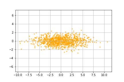
In order to get a good sense of what exactly is going on, we are going to apply the algorithm to a small dummy data set. This data set contains a thousand pairs of coordinates.

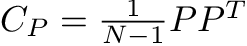
• cov_mat: the covariance matrix for this distribution (covariance matrix is explained in a bit)
• mean: the mean of the distribution
• size: number of data points to produce

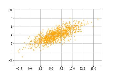
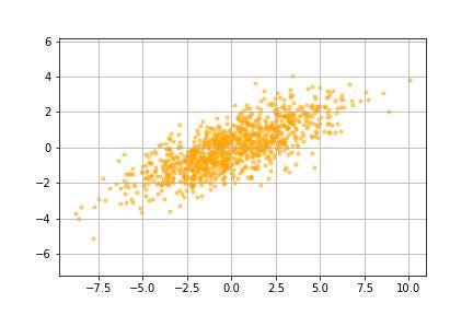
Next, we are going to center the data around the mean by subtracting the mean from all the data points. This also makes it easier to use linear algebra techniques since linear algebra is like things anchored at the origin.

Each datapoint can now be treated as a vector from the origin. We now need a way to encode some way of measuring ‘variance’ so that we can identify vectors along which it (variance) is maximized. To do this, we use the covariance matrix.

The two goals of the whole algorithm: maximize variance (to maximize the insights or signals from our data) and minimize redundancy, is encoded in the covariance matrix. The intuition behind this matrix is arguably the most important in order to get a sense of this algorithm.

Covariance measures the degree of the linear relationship between a pair of attributes. A large covariance value indicates a strong linear relationship, and a low value indicates a weak linear relationship. This means high values of covariance indicate a large degree of redundancy.

Given a multi-dimensional dataset, we need a way to keep track of the covariances between each of the pairs of features. Remember: covariance is how we encode the notion of redundancy, and variance is how we encode signal strength in our algorithm.

The covariance matrix, C, contains the covariance between each possible pair of attributes/features in our data set: for this data set with two features (x,y), the covariance matrix is 2X2 with four entries. Naturally, the diagonal entries in the covariance matrix capture the variances of each of the features/dimensions. The off-diagonal elements capture the covariance of each feature with every other feature.

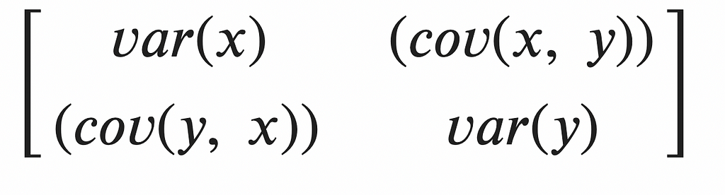
Maximizing signal (variance), and reducing redundancy (covariance) translates to maximizing the diagonal entries (the variances) and minimizing the off-diagonal entries. Our ideal data set would therefore have a diagonal covariance matrix!

So PCA aims to find a transformation matrix (A) to transform our (centered) data-matrix (Z) such that the resulting matrix, Z_pca, has a diagonal covariance matrix.

Linear Algebra makes finding such a transformation matrix very simple. It turns out that the eigenvectors of our covariance matrix of Z (mean-centered data) give us such a transformation.

Here is a picture of a brief proof :

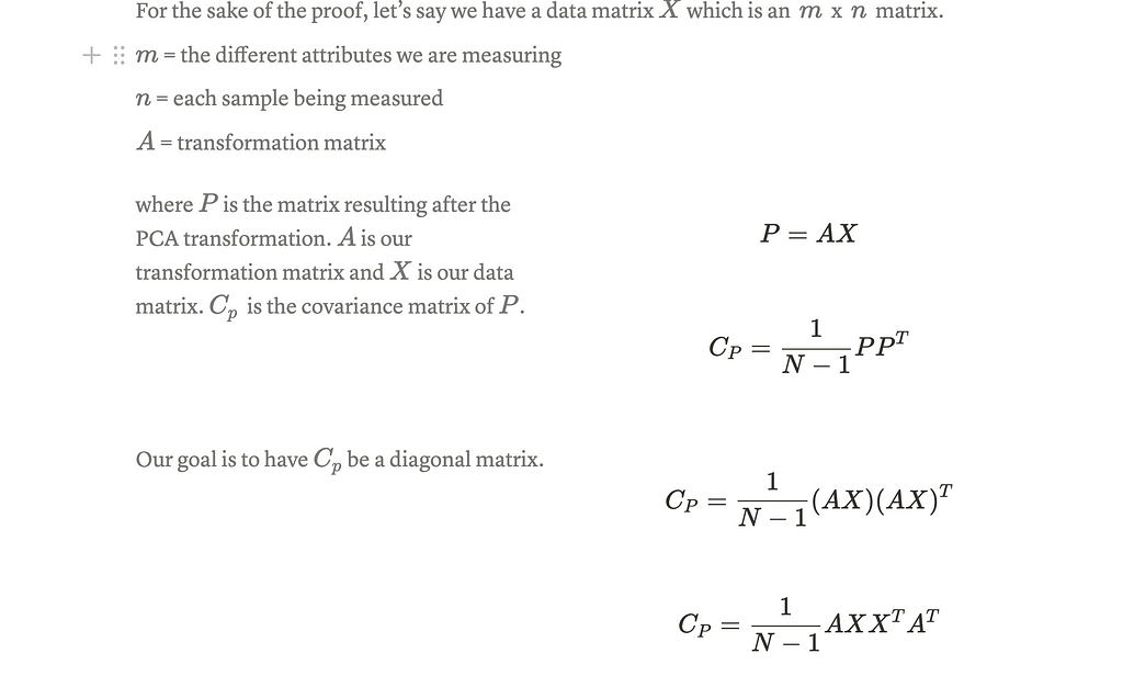
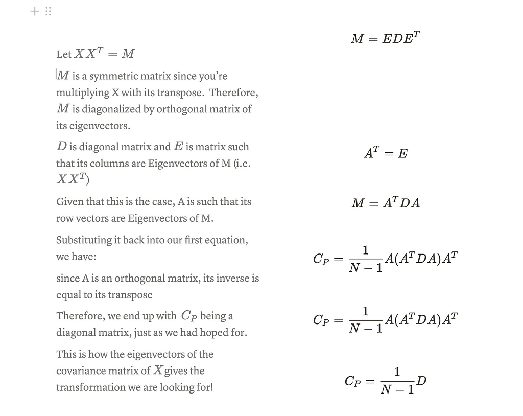
Note: the difference in the way the matrix is defined in the proof and while actually performing PCA. The way PCA literature defines the data matrix has the columns as the features being recorded and the rows as the samples.

The eigenvectors give us the direction of the principal components, while the corresponding Eigenvalues give us the ‘usefulness’ of each of the principal components (Eigenvectors).

Therefore, ordering the eigenvectors in decreasing order of their corresponding eigenvalues would give us the ideal transformation matrix.

what are eigenvectors?

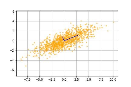
Now we actually apply this transformation matrix (multiply the transformation matrix to our data matrix) to our data to change to the new, more useful coordinate system.

And now we are done!!

We see that the data is now plotted relative to the eigenvectors (principal components) in image ___. To summarise the transformation:

• We first translated the data by subtracting the mean from the data
• We then rotated the data by an angle required to align the principal component axis (the eigenvectors) with the default x, y-axis

The link between PCA and SVD

Another way to perform PCA would be by taking advantage of its link with Singular Value Decomposition (SVD). We get to skip a few steps by using this approach!

Don’t worry if you have not done SVD before, you can still follow along and do the image compression portion. The important thing is to understand the covariance matrix from above, which is what helps us understand the intuition behind PCA works.

What is Singular Value Decomposition?

The key idea here is that the eigenvectors of the covariance matrix can be directly achieved through the Singular Value Decomposition of Z (our mean-centered data matrix).

SVD of our matrix Z decomposes the matrix as:

V is the orthogonal matrix whose columns are eigenvectors of Z.T * Z .

Therefore, the column vectors of V are eigenvectors of C, our covariance matrix!

Therefore, the rows of V.T give us the principal components! V.T is our transformation matrix!

You can use the code below to prove that this is true!

The singular values scaled by 1sqrt(n-1) measure the variance captured by each of the principal components.

Eigenvalues are squares of the singular values. And as mentioned before, eigenvalues give a sense of the variance captured by the corresponding eigenvector (principal component).

To determine the ratio of how much variance is captured by K number of principal components:

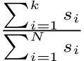
where s_i is the i-th singular value, k is the number of components being kept, and N is the total number of principal components.

To explore this method further, we are going to compress an image from the James Webb Space telescope.

Be sure to download this image and save it in your current working directory/folder.

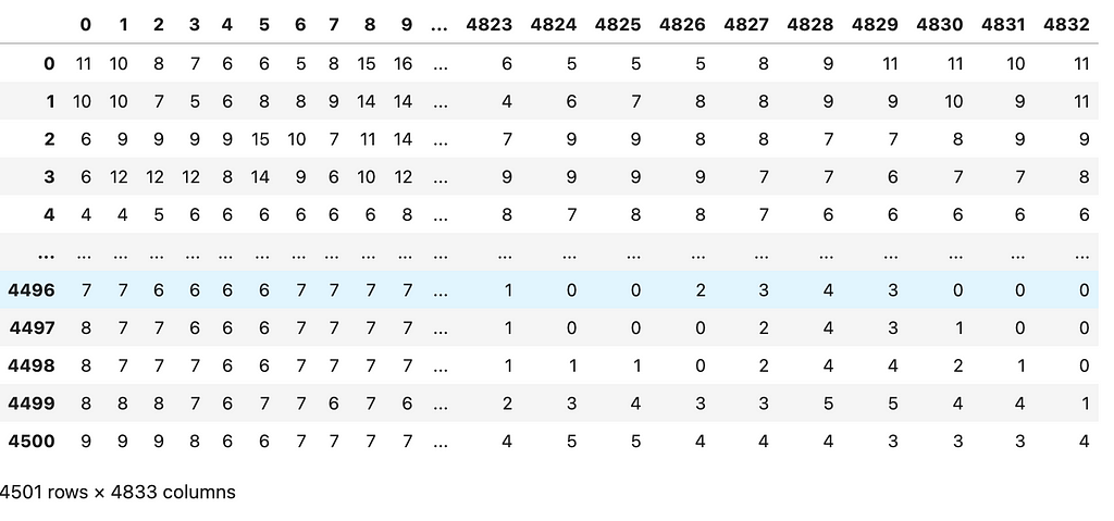
The shape of the array:

• we have three 4501 X 4833
• Each of the three matrices corresponds to the red, green, and blue image channels

We separate the three matrices. Each matrix (color channel) is going to be processed on its own.

To get a sense of what these matrices look like we can import one of them into a data frame.

The next step is to mean-center the data:

• calculate the mean row for each matrix
• subtract the respective ‘mean rows’ from all the other rows in each of these matrices

Now we perform Singular value decomposition on each of the Z matrices instead of calculating the Covariance matrix. This lets us skip a few steps.

The rows of Vtr, Vtg, and Vtb are the principal components of the respective data sets. They are ordered in terms of decreasing variance.

Now that we have our principal component matrix — the transformation matrix — we are almost done. All we have to do is apply the transformation (multiply the Transformation matrix by our respective Z matrices)

We can now use this image to demonstrate a cool use case of PCA: dimensionality reduction (image compression). For this, we have to decide how many principal components we want to retain. We can decide this by looking at the ratio of the sum of K singular values to the sum of all singular values as defined earlier. We can also eyeball it and play around with the number of principal components until we are satisfied with the final (uncompressed) image.

This image is from the 400 principal components we stored! 400 principal components stored 80% of the variance according to the ratio of singular values.

The resulting image:

While there are better methods for image compression, this is a fun way to demonstrate one of the most popular uses of PCA: dimensionality reduction.

The Summary:

• PCA is a data-transformation technique
• The idea is to get better insights from our data by using a different coordinate system
• PCA is super useful for dimensionality reduction, particularly if you don’t want to delete any of your original attributes explicitly
• PCA picks the new set of dimensions/axes based on the directions of variance in your data.
• Variance is captured by the Covariance matrix.
• Eigendecomposition of the Covariance matrix results in the new set of dimensions — the principal components.
• The principal components are linearly independent and orthogonal to one another. They are also ordered from the most important to the least important based on the amount of variance they capture

Resources For Additional Study/Exploration

• The Jupyter notebook: https://github.com/tenglina/PCA
• Eigenvectors and Eigenvalues: https://www.youtube.com/watch?v=PFDu9oVAE-g&t=466s
• Singular Value Decomposition: https://www.youtube.com/watch?v=EfZsEFhHcNM&t=1s
• PCA and SVD: https://www.youtube.com/watch?v=DQ_BkPHIl-g
• PCA using sklearn: https://www.geeksforgeeks.org/implementing-pca-in-python-with-scikit-learn/
• Visualize and learn PCA: https://setosa.io/ev/principal-component-analysis/
• Favorite Linear Algebra playlist: https://www.youtube.com/watch?v=J7DzL2_Na80&list=PL221E2BBF13BECF6C&index=3
• Great Linear Algebra playlist for intuition and visualization: https://www.youtube.com/watch?v=fNk_zzaMoSs&list=PLZHQObOWTQDPD3MizzM2xVFitgF8hE_ab

---

You’re Missing The Point Behind PCA was originally published in Towards AI on Medium, where people are continuing the conversation by highlighting and responding to this story.

Join thousands of data leaders on the AI newsletter. It’s free, we don’t spam, and we never share your email address. Keep up to date with the latest work in AI. From research to projects and ideas. If you are building an AI startup, an AI-related product, or a service, we invite you to consider becoming a sponsor.

Published via Towards AI