VectorDB Internals for Engineers: What You Need to Know

Author(s): Harsh Chandekar

Originally published on Towards AI.

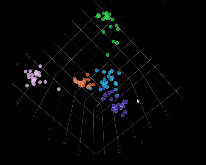
Ever wondered how your friendly neighborhood AI knows that “king” is somewhat similar to “queen” but definitely not to “banana”? The unsung heroes behind this magic are embeddings, and their meticulously organized apartments are vector databases.

Think of embeddings as the AI’s internal language — a super-dense, high-dimensional numerical representation of just about anything: text, images, audio, you name it. Words with similar meanings, or images showing similar concepts, are mapped to “nearby” points in this complex numerical space. But how do these magical numerical arrays get created, and how do they find their perfect spot in a database optimized for them?

The Architect’s Blueprint: How Embeddings Get Their “Spacing” (Loss Functions)

Before an embedding can move into its vector database pad, it needs to be “shaped” by a rigorous training process. This is where loss functions come into play, acting like strict architects ensuring that similar items live close to each other, and dissimilar ones are pushed far apart.

One of the most popular training methodologies for creating these intelligently spaced embeddings is Contrastive learning. This approach explicitly focuses on contrasting pairs of instances, making sure the model learns to capture relevant features and similarities within the data.

Contrastive learning comes in a couple of flavors:

• Supervised Contrastive Learning (SCL): This method uses labeled data to explicitly teach the model to differentiate between similar and dissimilar instances. It’s like having a detailed map, telling the model exactly which neighbors are friends and which are, well, not so much.
• Self-Supervised Contrastive Learning (SSCL): This is the unsupervised maestro. It learns representations from unlabeled data by designing clever “pretext tasks” to create its own positive and negative pairs. A common trick is to take an image, create several augmented (transformed) versions of it (like cropping or rotating), and treat these as positive pairs. Instances from different original images become negative pairs. The model then learns to differentiate between these “augmented views,” effectively capturing higher-level semantic information.

Now, for the architectural tools themselves — the loss functions that dictate this spacing:

• Triplet Loss: This is arguably the most famous and intuitively understandable loss function for metric learning. It operates on “triplets” of data points:
• An anchor instance (your reference point).
• A positive instance (semantically similar to the anchor).
• A negative instance (semantically dissimilar to the anchor).
• The goal of triplet loss is simple: The distance between the anchor and the positive must be smaller than the distance between the anchor and the negative, by a predefined margin. If this condition isn’t met, the model gets penalized. For example, in facial recognition, if your anchor is a photo of dog, the positive is another photo of dog, and the negative is a photo of dolphin. Triplet loss ensures that dog’s photos cluster tightly together, while dolphin’s photo is pushed far away.

• However, choosing these triplets isn’t always easy. Random selection often leads to “easy” triplets where the negative is already far away, providing little learning signal. This led to more sophisticated “mining” strategies:
• Hard Negative Mining: This strategy seeks out the most challenging triplets, specifically those where the anchor is more similar to a negative example than it is to its own positive example. These are the literal “errors” in the semantic mapping. While seemingly ideal, optimizing with these can lead to “bad local minima” during early training, essentially confusing the model and pulling dissimilar points closer together instead of separating them. It’s like trying to teach a child to ride a bike by only showing them videos of crashes — it’s informative, but perhaps too much, too soon!
• Semi-Hard Negative Mining: To avoid the pitfalls of truly hard negatives, this approach selects negative examples that are farther than the positive but still within the margin. It provides a challenge without derailing the training.

• Selectively Contrastive Triplet Loss (SCT): A newer, more robust solution designed to tackle the hard negative problem. SCT cleverly decouples the anchor-positive and anchor-negative pairs, essentially focusing the learning efforts on pushing only the hard negative examples away. This modification helps in situations where traditional triplet loss struggles, especially with datasets featuring high intra-class variance (e.g., different pictures of the same bird species looking quite different). The result? More generalizable features that are less prone to overfitting and more “spread out” in the embedding space. This means your AI can recognize “dog” better, even if it’s never seen that exact dog before!
• InfoNCE Loss (Information Noise Contrastive Estimation): A popular variant of contrastive loss, InfoNCE measures similarity by treating the problem as a binary classification task: given a positive pair and a set of negative pairs, the model learns to discriminate them. It’s widely used in self-supervised learning for its effectiveness.

• N-pair Loss: An extension of triplet loss that considers multiple positive and negative examples for a given anchor, providing more robust supervision. Just like the triplet loss but extended it to the n -pair instead of 3.

• Logistic Loss: Also known as cross-entropy loss, it’s adapted for contrastive learning to model the probability of two instances being similar or dissimilar.

These loss functions, in essence, are the guiding forces that carve out the meaningful, semantically rich spaces where embeddings will eventually reside.

The Digital Neighborhood: Storing Embeddings in a Vector Database

Once our embeddings are beautifully shaped and spaced by the training process, they need a place to live. Enter vector databases, purpose-built for storing, managing, and, most importantly, quickly searching these high-dimensional numerical vectors.

At their core, vector databases store embeddings as numerical arrays. The storage architecture typically involves two key components: the raw vector data (often compressed for efficiency) and a separate index that acts as a map for fast search operations.

But how do they find the “nearest neighbors” in a space that could have hundreds or thousands of dimensions? This is where specialized indexing structures come in, optimized for rapid similarity searches. Since exact nearest neighbor search is computationally impossible for large datasets with high-dimensional vectors (it scales linearly with data size and becomes very slow), vector databases rely heavily on Approximate Nearest Neighbor (ANN) algorithms. These algorithms trade a tiny bit of accuracy for blazing fast speed, which is perfectly acceptable for most real-world AI applications like recommendation systems.

Popular ANN indexing techniques include:

• Hierarchical Navigable Small Worlds (HNSW): Imagine a vast network of interconnected social groups. HNSW organizes vectors into layers of graphs, where higher layers allow for broad, coarse-grained navigation (like finding the right city), and lower layers refine the search to pinpoint the exact neighborhood (and house!).

• Inverted File Index (IVF): This method clusters vectors together, making it easier to search within specific clusters rather than across the entire dataset.

The Language of Closeness: Understanding Similarity Metrics

So, you’ve got your embeddings perfectly spaced and living in their optimized database. Now, how do you actually ask the database to find “similar” items? This is done using similarity metrics, which quantify the “distance” or “closeness” between two embeddings. The choice of metric is crucial, as it defines what “similar” truly means in your specific context.

Here are the main contenders:

• Euclidean Distance: This is the classic “straight-line distance” between two points in space. It considers both the magnitudes (lengths) and directions of the vectors. While straightforward, it’s less commonly used with embeddings from deep learning models and is more suited when the magnitude of the vectors inherently carries important information, like counts or measures.
• Dot Product Similarity: Calculated by summing the products of corresponding components of two vectors. The dot product is influenced by both the length and direction of the vectors. If two vectors point in the same direction, their dot product will be larger. Many Large Language Models (LLMs) are trained using dot product, making it a natural choice for their embeddings. If an embedding’s magnitude correlates with “popularity” or “strength,” dot product can capture this.
• Cosine Similarity: This metric measures the angle between two vectors, completely ignoring their magnitudes. This means vectors pointing in the exact same direction will have a cosine similarity of 1 (most similar), while orthogonal vectors will have 0, and vectors pointing in opposite directions will have -1. Cosine similarity is a go-to for semantic search and document classification problems, as it focuses purely on the “direction” or “topic” of the embeddings. It’s excellent when you care more about the qualitative “aboutness” of an item than its quantitative “intensity.”

The Golden Rule: The most crucial piece of advice for choosing a similarity metric for your vector database is simple: match it to the one used to train your embedding model. If your model was trained to optimize for cosine similarity, then using cosine similarity in your vector database will yield the most accurate results. If you don’t know, or if the model wasn’t trained with a specific metric, then experimentation is your best friend.

Beyond the Basics: The Joys and Woes of Scaling Vector Search

Storing and searching billions of high-dimensional vectors isn’t a walk in the park. Vector search faces significant scalability challenges:

• Computational Complexity: As datasets balloon, the resources needed for similarity searches skyrocket. Those high-dimensional vectors (like 512-dimensional embeddings) mean a lot of number crunching for each distance calculation.
• Memory Usage: Vector indexes themselves are memory hungry. A billion 768-dimensional vectors can easily eat up 3 TB of memory, far exceeding a single machine’s capacity. This is why distributed systems, which shard data across multiple nodes, are essential.
• Distributed System Design: While sharding helps, it introduces new headaches: maintaining consistency across nodes, handling node failures, and minimizing latency when querying across a vast, distributed network.
• Real-time Updates and Query Throughput: Imagine a recommendation system constantly learning from new user actions. Adding new embeddings requires continuous index updates, which can cause downtime or performance hiccups. High query loads (thousands per second) demand robust load balancing and caching.

Despite these challenges, vector databases are continuously evolving, with ongoing innovations in integration with AI/ML workflows, real-time analytics, and even future possibilities with quantum computing. They also often store metadata (like IDs, timestamps, or source data) alongside the vectors, typically in a hybrid setup with traditional databases, to provide rich context to search results.

In the end, embeddings are more than just numbers; they’re the semantic DNA of your data. Vector databases are the specialized homes that not only store this DNA but also allow your AI to quickly find its family members, enabling the intelligent applications we increasingly rely on. So next time your AI seems to “understand” you, give a nod to the humble, yet incredibly powerful, embedding and its dedicated abode in the vector database!

Thankyou for reading!

Join thousands of data leaders on the AI newsletter. Join over 80,000 subscribers and keep up to date with the latest developments in AI. From research to projects and ideas. If you are building an AI startup, an AI-related product, or a service, we invite you to consider becoming a sponsor.

Published via Towards AI