Taking Into Account Temporal Aspects of Machine Learning Apps

Author(s): Ori Abramovsky

Originally published on Towards AI.

Temporal features require special handling, from how to split the training population to the way to define the task at hand. In some cases, it can even mean overfitting on purpose.

Time-based splitting to prevent overfitting (except when it’s useful)

When developing machine learning models, one of the very first phenomenons to avoid is Overfitting; to make sure our models generalize well, that they don’t rely too much on the train data, and that they will be able to act well on new, unseen, data samples. A common relevant toy example is to mistakenly add an id feature when trying to predict if one will return a loan; on train data, it will probably be the most dominant feature (leading to a 100% accuracy, the model will just memorize the train samples) while on future records it will probably fail the model due to now facing different id values (the solution will be to add as features the loaner characteristics which are the real important data pieces that the id field represented). For applications with time-based aspects, avoiding overfit will mean verifying that the models have ‘changes robustness’; that they don’t rely too much on data step t in order to make them useful for data step t+1 as well. Consider, for example, a common website login count; most cases will have high values during the weekdays and low values on the weekends. Training a model to predict the next-day values using only the weekdays will fail due to overfitting to the samples in hand, and not being familiar with the weekends. Time base splitting can solve; by doing a train-test and k-fold splitting based on the time axis. Constantly verifying step t+1 to make sure the model didn’t overfit step t. On the other hand, in some cases, temporal overfit may be beneficial. A relevant example can be when trying to predict a customer request’s topic given its content. Many companies have their special jargon like ‘Slides’ or ‘Colab’ for Google and ‘OneDrive’ or ‘365’ for Microsoft. Such terms can be super useful in order to predict a request topic. To enable our models to leverage it, we should tune the Natural Language Processing practices in use in order to make sure these terms are visible (like not applying common NLP preprocessing techniques such as replacing digits with placeholders or using sub-words tokenization instead of word-based). An important drawback with such features is the fact they tend to be time critical. The term ‘Facebook’ for example, was probably an important indicator for many such developments, but one whose importance dropped the minute the new brand ‘Meta’ was announced. What we need in order to fix it is the ability to forget; to pay more attention to the recent terms. A solution can be to timely retrain our models in; first, by splitting the train population by time, we can easily identify that such discrepancies exist (like if the term ‘Facebook’ was super important on the train population but one whose importance vanished on the test population) and using K-fold by the time we can verify if short time overfitting could be beneficial. Finally, the implementation would be to periodically retrain with a vanishing factor, enabling our models to quickly tune to new terms (Meta) while not too quickly forgetting the old ones (Facebook).

Taking into account windows — Anomaly Detection labeling

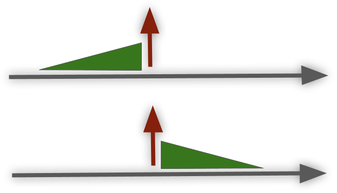
Anomaly Detection methods are commonly in use when supervised learning is not possible. Highlighting places where the data doesn’t behave in its normal ways, hiddenly assuming that such an anomalous behavior can indicate a higher likelihood of events of interest. Consider, for example, operational data like servers monitoring; the hidden motivation for applying anomaly detection tools here will be the assumption that anomaly alerts can indicate the existence of operational issues. But how to measure that assumption? How to correlate anomalies to failures? Moreover, as many operational issues will lack a clear input -> output relation (bad query can lead to database latency which can lead to the latency of a server which can finally lead to edge devices being stuck, but it’s difficult to draw the line towards the bad query which started it all). A possible solution would be to mark ‘relevance windows’ around target events, enabling us to measure if a given set of anomaly alerts could indicate them. It will be especially useful in order to tune the anomaly detection algorithms, deciding how critical an alert is, and in order to rank the importance of acknowledging these alerts. In our operational data example, we can highlight two main window types –

• Pre-windows; sudden incidents (power is down). Anomalies are likely to appear soon after the target event (the downtime).
• Post-windows; evolving incidents (servers upgrade generated deadlocks which eventually led to a downtime). Anomalies are likely to appear before the target event (the downtime), denser and denser as we get closer to it.

Such target correlations can be the main measure of how useful an anomaly detection tool is. Keep in mind though, that the results will highly depend on meta choices such as target events window size.

Labeling state while trying not to be too late

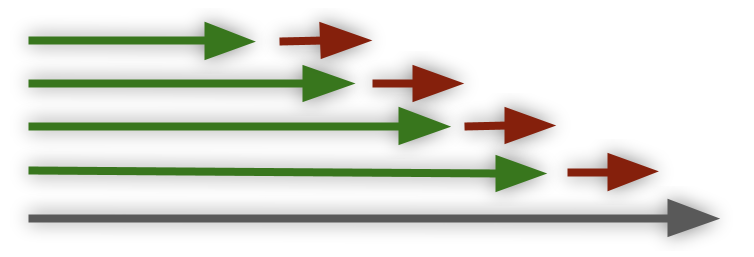
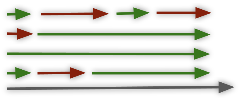
Another common temporal use case is to predict the state. Consider, for example, that we want to predict a customer state to auto-detect the ones which are likely to churn. Usage matrices are commonly the number 1# feature for that need, but how should we handle them? Different customers will have different lengths of historical values. Relying on aggregations (to make all customers’ historical values of the same size) can miss inner-aggregation insights (like sub-patterns that are not visible on the aggregated POV). Relying on fixed-size windows highly depends on the window size; too long windows can affect the ability to detect short churn, and too short windows can be too fuzzy, generating many false positive alerts. A common practice will be to set a minimum valuable time span, such as a quarterly usage frame as the population POV. The next question would be how to choose these quarters for the train population; customers’ initial quarter can be biassed towards the fact it takes time to fully utilize new products, customers’ last quarter (before churn) can be biassed towards the fact they are already in the middle of transitioning elsewhere. Such choices are even more critical given that our main motivation was to prevent churn, and if we are good only at highlighting churn candidates the minute before they leave (at an un-savable point in time), then our solution won’t be of any use. A common technique to verify the settings in use is to check how beneficial the output was — given that X ‘in risk to churn’ alerts were generated, for how many of them the churn was prevented. Keep in mind, though, that such a solution will require us to avoid an important, relevant pitfall — the hidden feedback loop; Assuming that following the previously mentioned advice, we decided to periodically retrain our model, on train cycle t+1 the data state may be affected by the model cycle t; ‘no churn’ scenarios can be due to reach-out teams successfully preventing churn using our alerts. Meaning that our updated data state can confuse the model, having scenarios that in the past indicated churn but not anymore (since now having the churn alerts). The solution should be, starting from retraining step #1, to add as a feature if an alert was made and what actions were taken following it to make it visible for the later model retrain iterations.

Forgetting on purpose bad data states

When developing supervised machine learning models, the first and most important ingredient is a labeled dataset, looking at past records in order to predict future ones. But an important note to make is that for some cases; the past will include bad samples, ones we would like our model to ignore in order to make it better. Consider, for example, a recommendations app that was generated by looking at the customers’ past purchases. Let’s assume the model decides that having product X is a super important indicator that the customer should have product Y as well, leading towards an immediate conclusion that customers having product X should be suggested with product Y. But digging into past records may reveal many relevant biases; we may find that for a long period of time, product Y was given for free to X buyers, or that it was suggested to every X buyer, or just that there was a defect-making product Y being always suggested to all customers. Such discrepancies can be easily identified using techniques like the ones we mentioned before; train-test splitting by time could easily identify biassed points in time. The solution should be to embrace a deeper, less naive POV. For some cases, we may even decide to ignore data of specific time spans (like customers purchasing product Y during the 100% discount period), assuming them to be nonrelevant to future cases. It’s important not to take past records as is but to try to understand if outer parallel biases may exist, ones we should remove from our train population. In our previous example, comparing the cancellation rates with the purchase rates could highlight that a hidden bias exists.

The importance of using time-critical techniques

As we’ve just seen, time aspects can affect machine learning models in various ways. The best approach is to assume that all data is time affected. It doesn’t necessarily mean that applying techniques like train splitting by time will be mandatory, but it does mean we should spend time during our data exploration phases verifying if time biases exist and if they do — making sure to prevent them.

Join thousands of data leaders on the AI newsletter. Join over 80,000 subscribers and keep up to date with the latest developments in AI. From research to projects and ideas. If you are building an AI startup, an AI-related product, or a service, we invite you to consider becoming a sponsor.

Published via Towards AI