MLOps Notes 3.2: Error Analysis for Machine learning models

Author(s): Akhil Theerthala

Originally published on Towards AI.

Hello everyone!
This is Akhil Theerthala. Another article in the MLOps series has arrived, and I hope you enjoy it. We’ve examined the phases of a Machine Learning project, got a high-level view of deployment best practices, and are now diving into the modeling best practices. If you have missed the previous article detailing the modeling (3.1), you can read it here.

Following up on our previous discussion, here, we’ll talk about the model’s error analysis and the difficulties and best practices that come with it.

Why do we even need error analysis?

Before diving, let us take a step back and ask ourselves the question ‘why’. Let’s say we have trained a machine-learning model. Now, we somehow need to evaluate its performance. This evaluation is generally done by traditional metrics like accuracy, which determines whether the model is worth something.

We mostly won’t get the best performance when we train a model for the first time. We, more often than not, get a model with a bad performance or an average performance. So how do we tweak the original architecture to achieve our ideal performance and build something useful?

Error analysis helps us meaningfully break-down the performance of the model into groups that are easier to analyze and help us highlight the most frequent errors as well as their characteristics.

To look at the standard practices involved, let us go back to the speech transcription model we discussed in our previous articles. In the speech transcription model, we have seen noise from different areas like vehicles, people, etc. How do we analyze the model performance and find areas of improvement?

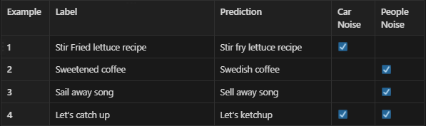
One way of analysis is to manually tag the samples under different categories and find the class with the highest scope of improvement, i.e., going through the examples manually and annotating them in a spreadsheet. In this speech transcription project, we take the labels and predictions for our model and try to recognize what kind of noise confused the model.

For simplicity, let us tag only 2 kinds of noise, one made by cars, and the other is the noise made by surrounding people. Then, we get the spreadsheet as the following table,

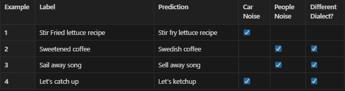
We might find other tags that can influence the errors during the analysis that we haven’t even considered initially. In our case, some of the errors might be due to the speaker’s low bandwidth or different dialect, etc. In such cases, the new categories are then identified and tagged correspondingly. This is shown in the following table,

This process aims to develop some reasoning as to what’s causing the errors and then productively improve the algorithm based on the reason. We can consider some of the following significant metrics to form the reasoning.

• What fraction of errors have that corresponding tag?
• What fraction is misclassified or mistranscribed of all the data with that tag?
  – This fraction gives us the performance of the data in that corresponding category and also tells us how hard the performance improvement can be.
• What fraction of the data has that tag?
  – This tells us how vital the examples with the tag are in the complete dataset.
• How much room for improvement is there on the data with that tag?
  – This is based on the baseline that we decided for the model. In our case, it can be the human-level performance of the model.

How to prioritize what to work on?

One common thing we have heard up to now is to work on the category with the highest scope for improvement. But how to identify this scope of improvement? Are there any pre-defined rules for that?

The answer would be NO. There are no pre-defined rules to decide what we should work on. But based on the earlier questions, we can get a general idea of what we can work on. So, to describe a situation in the above model we defined, let us consider the following table,

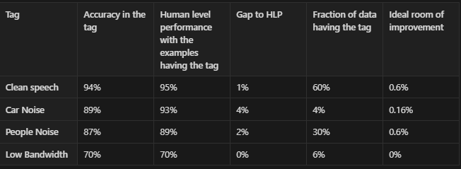
The ideal room of improvement gives us the percentage of improvement we get if we try to match the human-level performance. In the case of clean speech, ideally, we can see a 1% improvement over 60% of data resulting in about 0.6% of performance improvement. Similarly, the calculations are done for all the tags that were identified. For our example data, this suggests we work on People’s Noise or Clean Speech to improve our model.

We can also add a new column indicating how vital a tag is to our model. For example, improving performance on the samples with car noise might be helpful when our target customers enjoy driving more than other activities. In that case, we need to add more data for that specific category and focus on improving the performance.

Working with Skewed Datasets.

Till now, we have seen the models generated on standard datasets. Other than these, we also have models where we need to work on skewed datasets and perform error analysis. We might develop a model for a factory where 99.7% of produced goods have no defects and only 0.3% have flaws. Or we could build a medical diagnosis system where 99% of the patients don’t have the disease.
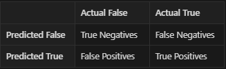
In these cases, we don’t use accuracy. Instead, we will build a Confusion matrix and calculate Precision and Recall for the predictions. The confusion matrix typically is a 2×2 matrix that generally has the model predictions along one axis and the true labels along the other axis. The following image describes a typical confusion matrix.

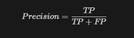
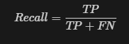
Using the values in the confusion matrix, we might also form different metrics and use them. Some of the metrics are precision and recall.

Precision: The proportion of true predictions that are actually true.

Recall: The proportion of actual true predictions that are identified correctly.

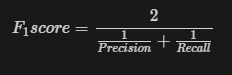
Since we have to constantly monitor these 2 metrics each and every time, some hybrid metrics, which alert when even one is not suitable, are defined by combining these two metrics. One of the standard metrics is the f-beta score, the weighted harmonic mean of precision and recall, reaching its optimal value at 1 and its worst value at 0.
The most commonly used f-beta score is the f-1 score, where we give equal weights to precision and recall.

So far, we have only seen the metrics for binary classification problems. But there are different ways to use these metrics for multi-class metrics. One way is to find the metrics independently for each class and use them to evaluate the model, i.e., consider each class as a binary classification.

Performance Auditing

Even when the model is performing well in training metrics and error analysis, it is recommended to do one final performance audit before sending it to production. There are many ways an audit might be performed.

One framework to audit your model is as follows.

1. Brainstorming the ways the model can go wrong like
2. Performance on the subsets of data,
3. How common are specific errors?
4. Performance on rare classes, etc.,
5. After identifying how the model can go wrong, you can establish metrics to assess performance against these issues.
6. After establishing these metrics, we can manually evaluate them or use different automated MLOps tools for auditing this performance.

Until now, this manual process is preferred, however, in the recent times there are emerging MLOps tools that helps us easily identify different kinds of errors. At the end it is up to the preference of the users.

With this, we have finished going through the error analysis of the machine learning models. Now, there is one last step left to explore in the modeling phase of a project, which is the data-driven approach to modeling. I am working on this article currently, and you can expect it before the same time, next week.

In the meantime, if you want to read my notes on CNN, you can read them here, or if you still haven’t read the last part of MLOps notes, you can find them here or in the links provided below. Thanks for reading!

P.S. you can subscribe using this link if you like this article and want to be notified as soon as a new article released.

• MLOps Notes -1: The Machine Learning Lifecycle
• MLOps Notes 3.1: An Overview of Modeling for machine learning projects
• Join me in my journey through Machine Learning…

---

MLOps Notes 3.2: Error Analysis for Machine learning models was originally published in Towards AI on Medium, where people are continuing the conversation by highlighting and responding to this story.

Join thousands of data leaders on the AI newsletter. Join over 80,000 subscribers and keep up to date with the latest developments in AI. From research to projects and ideas. If you are building an AI startup, an AI-related product, or a service, we invite you to consider becoming a sponsor.

Published via Towards AI