Medical Image Segmentation: 2018 Data Science Bowl

Last Updated on January 6, 2023 by Editorial Team

Last Updated on November 2, 2021 by Editorial Team

Author(s): Kriz Moses

Deep Learning

A case study on Nucleus Segmentation across imaging experiments using Deep CNNs (UNet, UNet++, HRNet)

Table of Contents

1. Abstract
2. Introduction
   – Problem Statement and Dataset used
   – ML Formulation of the Business Problem
   – Real-World Constraints
   – Metric used
3. Literature Review
   – Challenges of medical image segmentation
   – Sliding Window Method
   – UNet
4. Exploratory Data Analysis
5. Deep Learning Architectures Used
   – UNet
   – UNet++
   – HRNet
6. Results and Discussion
7. Post-Training Quantization
8. Web Application
9. Summary and Future Work
10. Acknowledgments
11. References

Abstract

To find the cure for any disease, researchers analyze how the cells of a sample react to various treatments and understand the underlying biological processes. Identifying the cells’ nuclei is the starting point for most analyses since it helps identify each individual cell in a sample. Automating this process can save a lot of time, allowing for more efficient drug testing and unlocking the cures faster. In this case study, I propose the use of Deep CNNs for the automation of nucleus detection in images across varied conditions. I design a total of three networks derived from U-Net, U-Net++, and HRNet and compare their performances using Mean IoU as the metric. It’s seen that U-Net based model performs the best with a Mean IoU score of 0.861.

Introduction

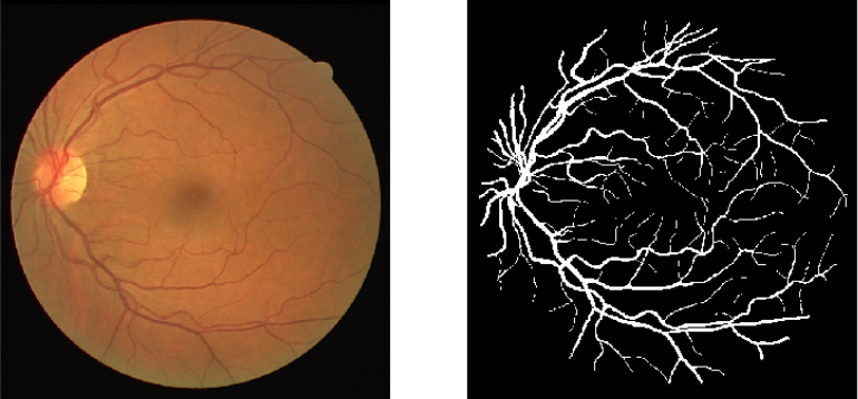
Image Segmentation is segmenting particular regions of an image for better understanding and analysis. For example, in the field of the medical domain, in a brain scan, doctors might want particular regions to be highlighted (which can’t be observed by the human eye that easily) for better diagnosis. Another application would be in a self-driving car when you need to segment different kinds of objects in the image. Below is shown an example of segmentation of blood vessels in retinal images.

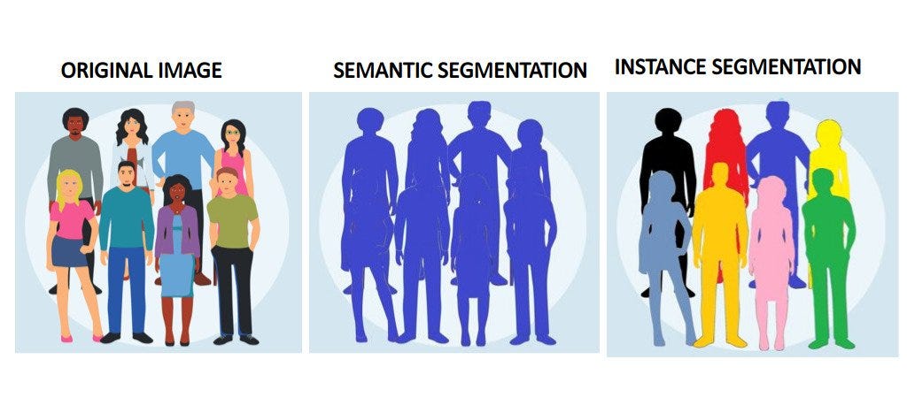
In general, there are two types of segmentation: Semantic and Instance. In Semantic Segmentation, different classes of objects are segmented separately (eg. separating people from background). Whereas, in Instance Segmentation, different instances of the same class are segmented (eg. separating different people from each other in the same picture)

Real-World Problem Statement and Dataset used

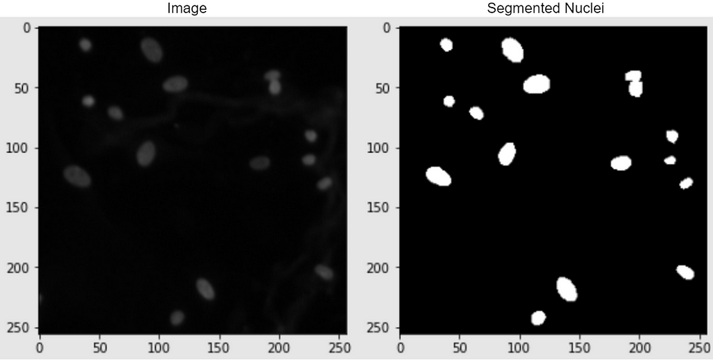
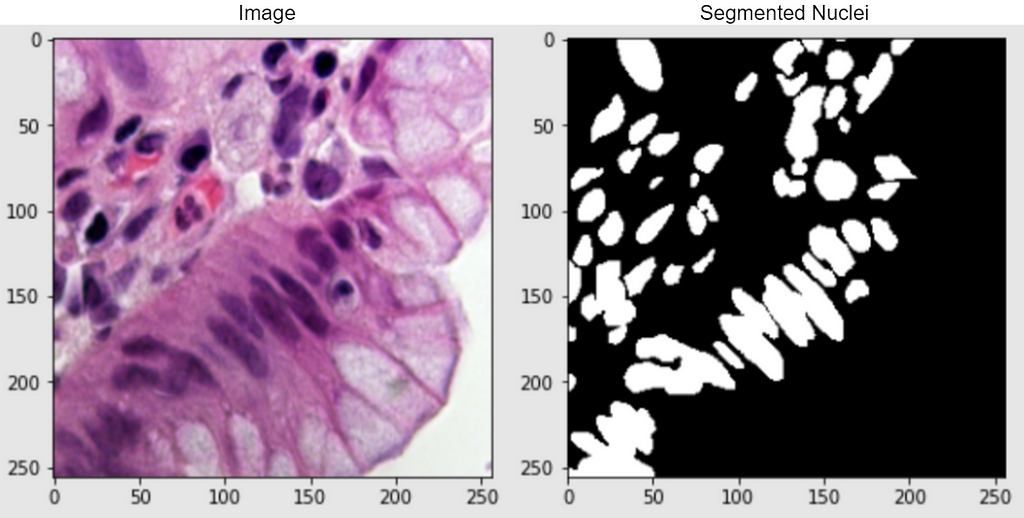
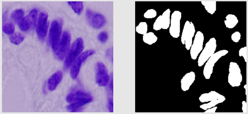
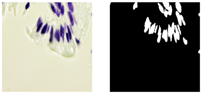
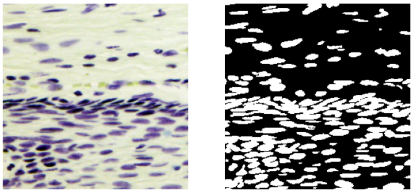
In this case study, I strive to solve a semantic-based medical segmentation problem. The dataset used is from the Kaggle competition 2018 Data Science Bowl. This has been used as a benchmark dataset for U-Net++ and DoubleUNet. The dataset consists of images of nuclei in different background conditions. The task is to segment the nuclei from the background. Below are shown a couple of examples from the dataset, of the image and its segmented nuclei mask.

Real-World Importance: The task that I will try to solve is to automate nucleus detection. This can help in speeding up research and getting the cure for almost every disease, from lung cancer and heart disease to rare disorders. This is because identifying nuclei is the starting point for most analyses because most of the human body’s 30 trillion cells contain a nucleus full of DNA, the genetic code that programs each cell. Identifying nuclei allows researchers to identify each individual cell in a sample, and by measuring how cells react to various treatments, the researcher can understand the underlying biological processes at work [2].

ML Formulation of the Problem

In general, image segmentation can be also posed as a multiclass classification problem in which every pixel in the image has to be assigned a class. Notice that here the input and the output are both images. Here, my input data point would be the image of the cells, and the output data point would be its segmented nuclei mask. The output image is labeled by an expert in the field. For our problem, the output image is a binary image with a background as black and nuclei as white.

So now given an input image (say of shape HxWx3), the task is to produce an output binary image (shape HxWx1) of the segmented nuclei i.e. to assign a binary number of 0 or 1 to every pixel of the output binary image.

Real-World Constraints

In the real-world, segmentation of biomedical images is considered to be really important for diagnosing purposes. And in a number of cases, a small error can lead to a false diagnosis which might put the health of a patient to huge risk. However, in our case, since the segmented nuclei would be used more for a general cure, hence small errors should not be as big an issue.

As far as latency is concerned, the segmented images of the nuclei do not need to be produced in milliseconds. A few seconds, even minutes should not hurt in most situations.

Metric Used

The metric used is Mean IoU i.e. the Mean Intersection Over Union.

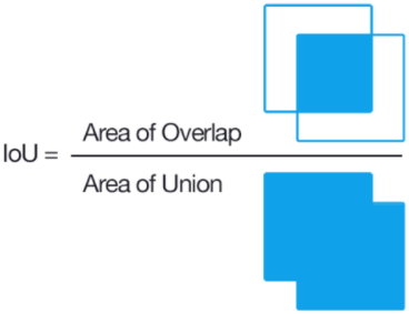
Its a very commonly used metric along with dice coefficient. The mean IOU for two objects can be defined as the area of intersection between them divided by the area of union. In image segmentation, the two objects are the true region and predicted regions of the part to be segmented.

To explain this better, say our object to be segmented is a football. Here the first object is the region of football in the real image. And the second object will be the region of the football in the predicted image.

So what does “Mean” signify in “Mean IoU”? “Mean” in “Mean IoU” stands for the average of all the classes to be segmented. So say in a task we need to segment all the cats from the background. So this task can be explained as a binary classification task, the two classes being a cat and the background. So mean IoU would be calculated by IoU(cat) + IoU(background) / 2

Similarly for multiclass classification,
Mean IoU = (IoU(class1) + IoU(class2) ….. + IoU(classN)) / N

Taking the mean of all classes helps to reduce the effect of data imbalance. A detailed explanation of Mean IOU can be found here.

Literature Review

Challenges of medical image segmentation

The task of Image segmentation in itself was a challenge for deep learning methods since the output of the network has to be an image as well. Typical CNNs take in an image as input and output a number. Here, we had to output an image. On top of that, in medical image segmentation, the problem became even tougher since the number of training images was very less. Hence the task is pretty challenging given the scarcity of data.

The traditional methods for solving this task include thresholding and clustering-based approaches. Over the last few years, a lot of development has been done in the field of deep learning for medical image segmentation.

Sliding Window Method

In this method, each pixel in the output image is predicted individually. The input fed for that every pixel is the cropped image of the surrounding (say 64×64) grid around that pixel. Thus, for every image (HxWx3), we have a total of HxW separate outputs and a 64x64x3 patch of the input image as input for each output. This method was very trivial in its time but then had a lot of disadvantages. 1) This method was very time-consuming at runtime and there was a lot of redundancy due to overlapping patches. 2) When using larger patches to preserve the global structure, a lot of max-pooling was to be used which failed in preserving the local structure, and for smaller patches, although localization was better the global context was lost.

U-Net

One of the pioneer papers in this field introduced a very unique architecture for this very problem, called U-Net. The architecture of U-Net is shown below.

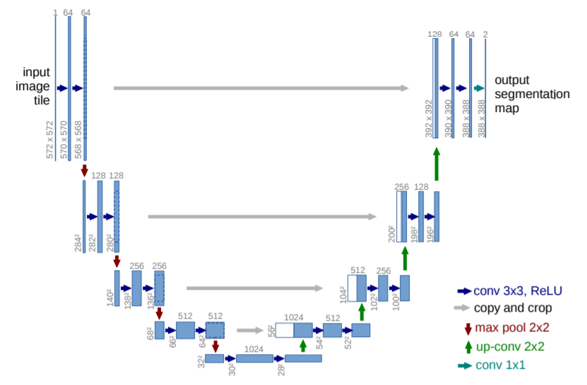
U-Net is an encoder-decoder type model, ensuring that both the input and the output are images. The encoder part of the architecture is normal convolutions + max pool and we eventually get to a very small size feature map. This part of the network tries to capture all the information about the image in a map of a small feature size. Now, this map is fed to the decoder part which tries to unravel the information and then get the desired output. Here, to get near the output image, the size of the feature map needs to increase while decreasing its depth. For this, we use up-conv (up sampling + conv). While using max pool local info was lost and up-conv does not help to retrieve that, hence to provide that information we use crop + copy from the previous map at the same horizontal level. The final output contains two maps. One for background and one for membrane. There is no padding used anywhere in the paper.

U-Net did really well with very few training images (30) from the EM Segmentation challenge. It improved the sliding window in two ways: skip connections and upsampling. Via upsampling, we no longer had to do pixel-wise segmentation and sacrifice the global context (as in the sliding window). And the skip connections help retain the local context lost while max pooling.

Since the introduction of U-Net, a number of successful architectures have been proposed which build on top of this as the backbone. In this case study, I have compared the performance of three models: U-Net, U-Net++, and HRNet. The architectures of the latter two are explained in the “Deep Learning Architectures used” section.

Exploratory Data Analysis

The dataset consists of images of cells in different background and their corresponding masks of segmented nuclei from the background. The competition was in two stages. For training, a total of 670 images and corresponding masks were provided. Stage 1 test set contained 65 images, and stage 2 test, 3019 images. The masks were provided for the stage 1 test images but not the stage 2 test. Hence in this case study, I use the 670 stage 1 train images as it is for training and the 65 stages 1 test images as the validation images. The masks for the stage 2 test are not provided, hence we can only use them for some manual analysis of how our model is working on unseen data.

So all in all, in this case, study, I use 670 images for training and 65 for validation. 3019 test images (without masks), will only be used for some manual analysis. A few examples are shown below consisting of the images and their masks.

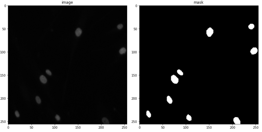
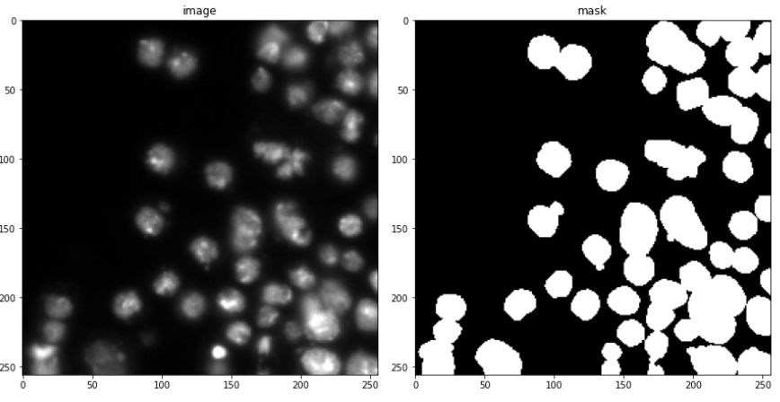
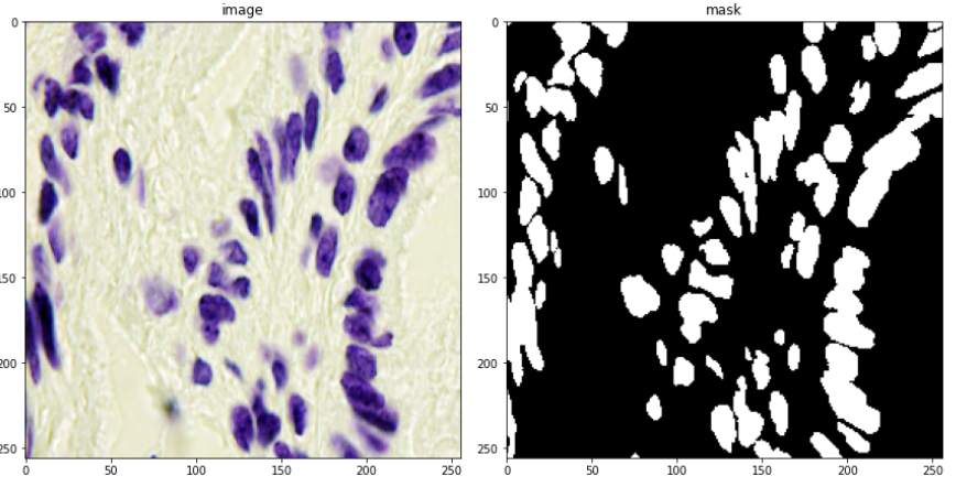
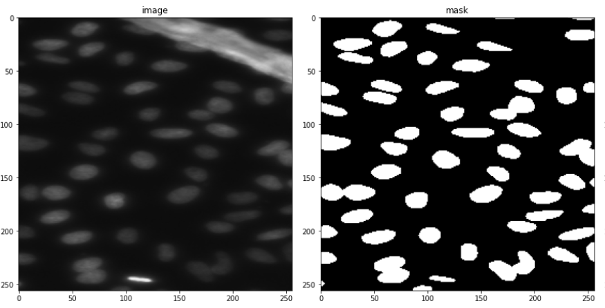
Looking at only the first two images, you might think, that this can be easily solved through simple thresholding, but that is not the case since the images contain a lot of variety of backgrounds. This is evident looking at the next two. This was the challenging part of the competition. Also what made it more interesting was that the validation images had a lot more variation in images than the train images. So a model had to be designed which can generalize well and not overfit the training set.

Dataset Details

The following observations were found after some basic data analysis:

• The images are found in different shapes, the most common being 256×256
• There are two types of images found in train and Val data: RGB and RGBA (4 channels). The last channel is called the alpha channel which decides the transparency (255 being opaque and 0 being transparent). Removing this channel will convert our image into an RGB image.
• On close inspection of test data, I found that there is only one image rare grayscale which is a grayscale image. Rest all other images are either RGB or RGBA.
• Images are found in different sizes.
• All images are on a 0–255 scale only. No image is found to be on a 0–1 scale.

Train Images examples:

• In train data, most images are black and white. Some are colored. The black and white images look easy to segment from the human eye. The colored images are generally purple in color. The train images don’t have a lot of variation in them.

Below are shown some train images examples with the image on the left and its a mask on the right.

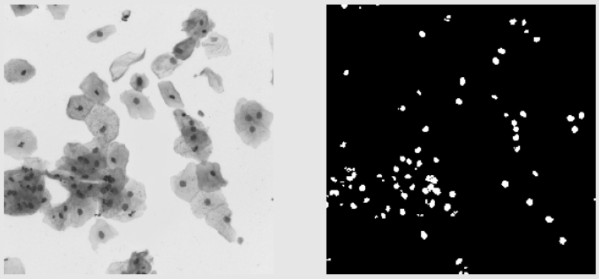
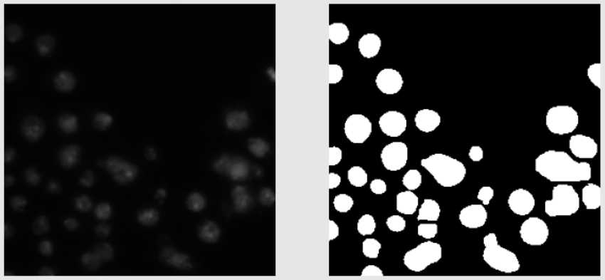
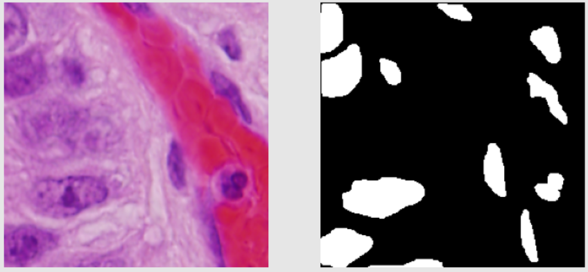
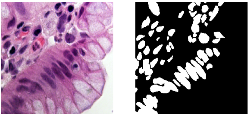
Validation Images Examples:

• The validation images seem a little harder to segment as compared to the training images. Some images are similar to the images from the training data and some are very different as seen below.

Validation Images Examples:

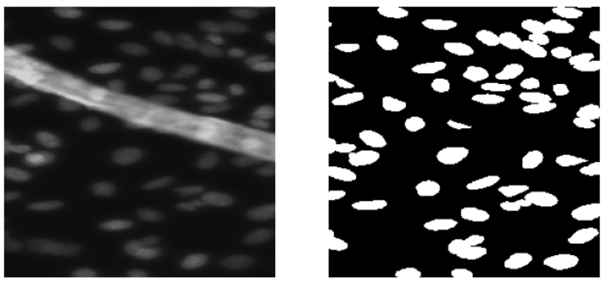
• The test images on the other hand contain a lot more variations. Below some examples of test images (no mask) are shown.

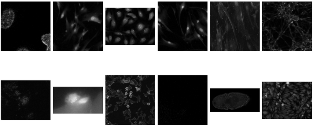
• Thus, the general observation is that the variation in images increases from train to validation to test. Hence, the chances of overfitting are higher, and thus the ability of the model to generalize is a very important part of the model building.

Deep Learning Architectures used

I have compared the performance of three models: U-Net, U-Net++, and HRNet. I decided the input and output shape of the images to 256×256, since that was the most common shape found, and is a pretty standard input shape in state-of-the-art CNN networks.

U-Net

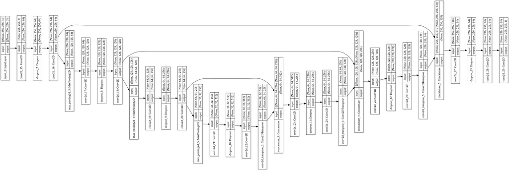
The architecture of the model is already explained in the “Literature Review” section. Unlike the standard U-Net with four encoder and decoder blocks each, I kept three of each. For up-sampling, I used the Conv2DTranspose layer. The whole code is written in Keras with Tensorflow backend. The code for U-Net, with the model image, is given below.

U-Net++

In U-Net, the two main ideas were skipped connections and up-sampling. Via up-sampling, we no longer had to do pixel-wise segmentation and sacrifice the global context (as in sliding window). Whereas the skip connections help retain the local context lost while max pooling. In medical segmentation, it is important to have as few errors as possible and capture the most minute of details possible. It is observed that skip connections have been very helpful in recovering fine-grained details of target objects; generating segmentation masks with fine details even on complex backgrounds. This is because the fine-grained low-level information is present in the actual image which gets coarser as we move down and right the network due to max pooling. And skip connections try to provide this information back to the decoder part when it’s trying to reconstruct the image. Without the skip connections the decoder really has no direct idea about the image, but only the final encoded map. With skip connections, the decoder gets to know the actual image and the fine details.

U-Net ++ builds on this and tries to refine these skip connections. U-Net combines deep, semantic, coarse-grained feature maps from the decoder sub-network with shallow, low-level, fine-grained feature maps from the encoder sub-network. And it combines them directly (crop and copy). U-Net2+ strives to enrich the encoder maps before combining them with the decoder maps i.e. make them more semantically (logically) similar before combining.

The architecture is inspired by Dense-Net. The advantages of dense-net are 1) Strong gradient flow 2) Fewer parameters and computational efficiency (The network is more complex and hence the network doesn’t need to be that deep) 3) Diversified features as each gets features from different layers.

The architecture of U-Net++ is given below. (The nodes capital X represent the conv operations and arrows represent the movement of feature maps. Small x i,j represent the outputs of the node X i,j)

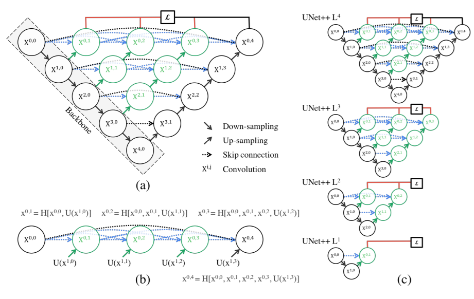
Two new concepts were introduced here: Dense Skip Pathways and Deep Supervision

Dense Skip Connections: Let x i,j denote the output of node X i,j where i indexes the down-sampling layer along with the encoder and j indexes the convolution layer of the dense block along the skip pathway. The stack of feature maps represented by x i,j is computed as:

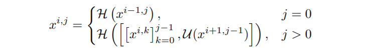
where function H(·) is a convolution operation followed by an activation function, U(·) denotes an up-sampling layer, and [ ] denotes the concatenation layer.

Notice that this is not only different in the way that we are using dense connections between encoder and decoder layers, but also that we are using convolutions instead of simply copying skip connections. In the original U-Net, they just copied. Apart from this the paper also uses deep supervision in which the outputs from all the top semantic layers are averaged.

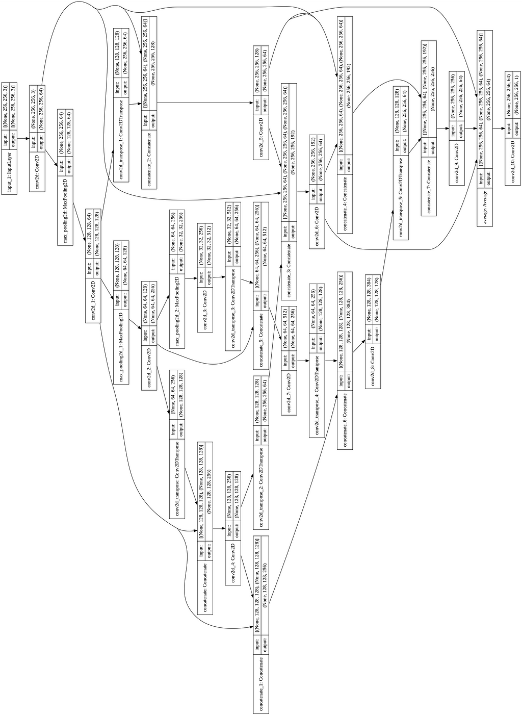
For its implementation, I reduced the number of convolutions in the encoder and decoder blocks by one layer. The code and the model image for the same are shown below.

HRNet
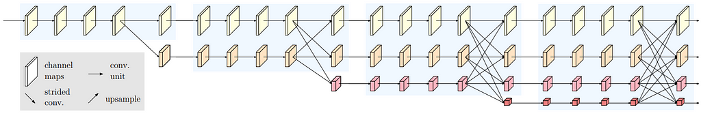
The network was inspired by this paper introducing a more densely connected architecture for segmentation, with the idea of extracting a deep representation of the different resolution features and then combining them together. Since the code and the image were pretty large in size, I did not include them here. You can find the code on my GitHub page.

Results and Discussion

All the models were trained with binary cross-entropy as the loss function. Adam optimizer was used, with a learning rate of 1e-3. I used early stopping with the patience of 20 epochs monitoring validation loss. For metric, I used a custom implementation of Mean IoU.

The graph for validation loss and Mean IoU is shown below

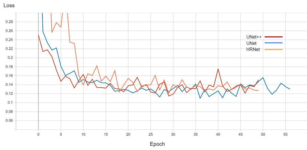
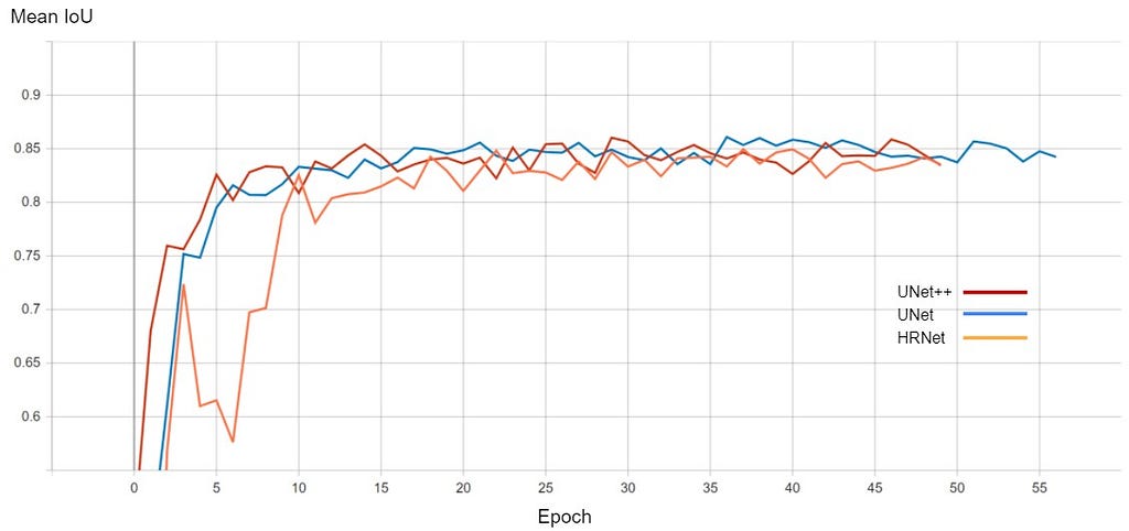
After training, for each model, the instance of the model at that epoch was selected which had the best Mean IoU. The comparison of all the models is shown below.

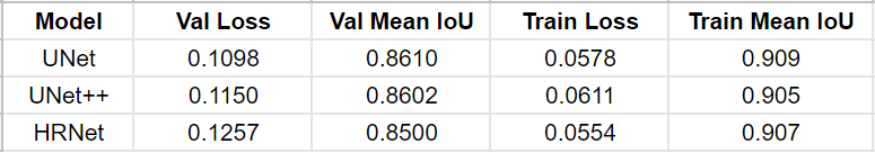
The performance of all three models is comparable. The training for every model stopped around the 50th epoch mark, meaning all had reached convergence around the 30–35 epoch mark. The best performing one was U-Net with a validation loss of 0.1098 and mean IoU of 0.861. U-Net++ was not far off with a score of 0.8602. HRNet had the lowest performance with a mean IoU of 0.85.

On top of this, I also experimented with increasing the number of encoder-decoder blocks for U-Net and U-Net++ but the models started overfitting and did not give any better results, hence I did not include them here.

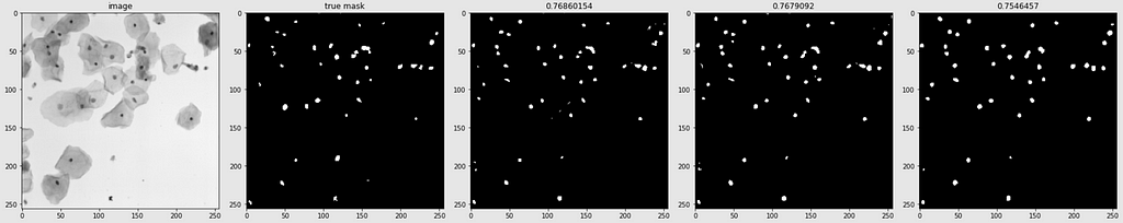
Predicted Masks

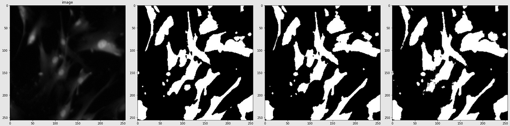
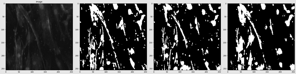
Below are shown the predicted masks for all the models with the Mean IoU score. Each row contains an image and a true mask followed by a predicted mask by UNet, UNet++, and HRNet in that order.

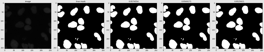
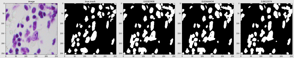
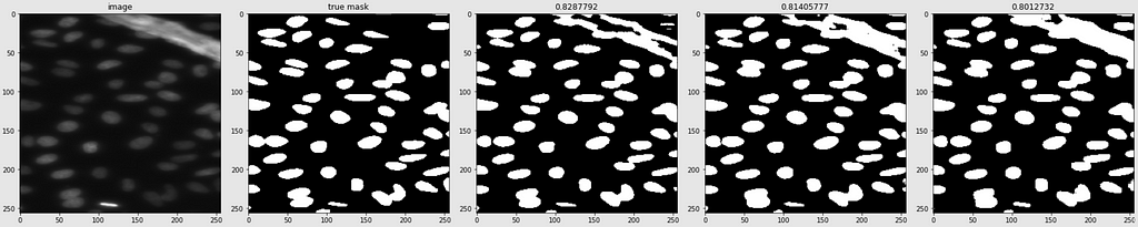
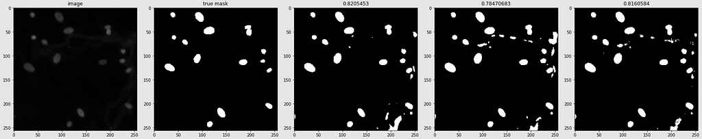
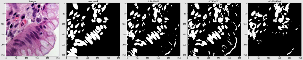
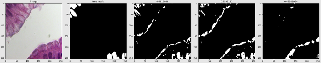
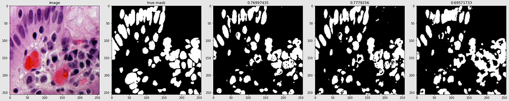
Below are some predictions on test images (without true masks and hence without scores)

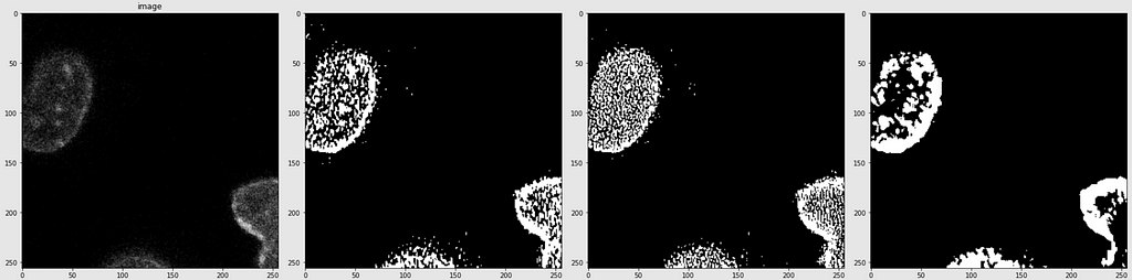
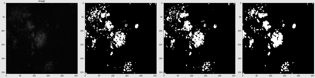
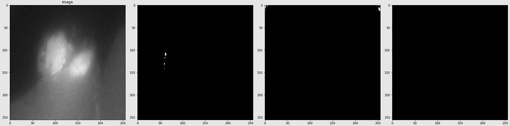
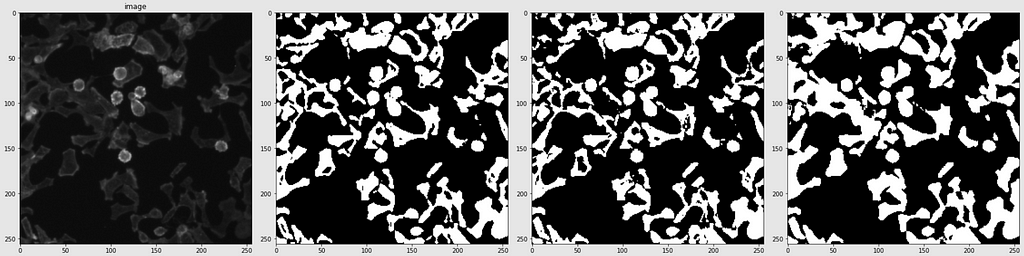
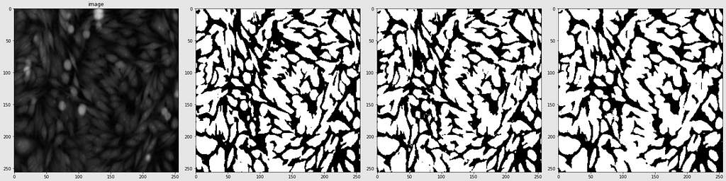
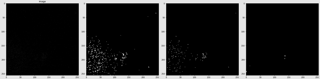
The performance of the models was quite decent for the validation images but the test predictions were not that satisfying. There is still the issue of generalization with such a few training images.

Finally, I selected the best model as UNet. The model had an average inference time of 0.964 seconds, with the model size being 28 MB.

Post-training Quantization

“Post-training quantization is a conversion technique that can reduce model size while also improving CPU and hardware accelerator latency, with little degradation in model accuracy.”
– TensorFlow Official Documentation

There are different methods for quantization. For my model, I used Float16 quantization in which all the weights are converted to 16-bit floating-point numbers. This reduces the model size by half: from 28 MB to 14 MB.

One important check-in quantization is to see if it does not reduce the performance of the model. This is the very reason I could not use other methods like dynamic range quantization, as these methods are not supported in the CPU in my box, and hence getting the outputs was taking a lot of time. Thus, it was not possible to examine if there is any degradation in performance. I could check for Float16 quantization, and there was no degradation in predictive performance (Mean IoU score was 0.861 for the quantized model as well) so I went with that.

So, finally, the model size was 14 MB. There was an increase in inference time from 0.964 seconds to 1.261 seconds, which is fine, given the decrease in model size.

Web App

I built a web app for this project and deployed it via streamlit:
https://share.streamlit.io/kriz17/mdt_app

Summary and Future Work

In this case study, I designed Deep CNN-based models for automation of nucleus detection in images under varied conditions. The performance of the total of three models was compared, which were based on U-Net, U-Net++, and HRNet. The best performing model was the U-Net-based one with a Mean IoU score of 0.861. Further, I used Float16 quantization to reduce the model size from 28 MB to 14 MB. The average inference time of the model was 0.126 seconds per sample which is decent for the task at hand. Finally, I deployed the model using streamlit.

All three models did a pretty decent job with each securing a Mean IoU score of greater than 0.85. They can be used for images with standard backgrounds as in the training data, but not with high variations. The main challenges were the small training dataset and the high variation in the backgrounds of the validation images. The conventional architectures of the models lead to overfitting, and hence I had to decrease the size of the models. In future work, I would like to try data augmentation using elastic deformation as implemented in the original U-Net paper. I would also like to explore Transformer Models based on attention mechanisms since they have proven to be really effective for small datasets [3].

Acknowledgments

I would like to thank the whole Applied AI Course team and especially Ramana Sir for guiding me throughout this case study.

References

[1] https://www.appliedaicourse.com/

[2] https://www.kaggle.com/c/data-science-bowl-2018/

[3] https://arxiv.org/pdf/2102.10662v2.pdf

[4] https://arxiv.org/pdf/2009.13120.pdf

[5] https://medium.com/swlh/image-segmentation-using-deep-learning-a-survey-e37e0f0a1489

[6] https://paperswithcode.com/task/medical-image-segmentation

[7] https://en.wikipedia.org/wiki/Image_segmentation

[8] https://arxiv.org/pdf/1505.04597v1.pdf

[9] https://towardsdatascience.com/review-u-net-biomedical-image-segmentation-d02bf06ca760

[10] https://drive.google.com/file/d/1U-SEtD5NExw86Bau7mOW9Lz9F1n7LpF3/view

[11] https://arxiv.org/ftp/arxiv/papers/1802/1802.06955.pdf

[12] https://arxiv.org/pdf/1802.02427.pdf

[13] https://arxiv.org/pdf/1807.10165v1.pdf

[14] https://arxiv.org/ftp/arxiv/papers/2004/2004.08790.pdf

[15] https://sh-tsang.medium.com/reading-unet-3-a-full-scale-connected-unet-medical-image-segmentation-ebb5e7f53caa

[16] https://arxiv.org/pdf/1908.07919v2.pdf

Full work with code can be found here on my GitHub profile:

GitHub – kriz17/Medical-Image-Segmentation

Connect with me on LinkedIn:

Kriz Moses – IIT Indore – Indore, Madhya Pradesh, India | LinkedIn

PS: Feel free to provide comments/criticisms if you think they can improve the project/blog. I will definitely try to make the required changes.

---

Medical Image Segmentation: 2018 Data Science Bowl was originally published in Towards AI on Medium, where people are continuing the conversation by highlighting and responding to this story.

Published via Towards AI