Fixing SimCLR’s Biggest Problem — BYOL Paper Explained

Author(s): Boris Meinardus

Originally published on Towards AI.

How BYOL introduced the new SOTA idea of all modern Self Supervised Learning frameworks.

SimCLR successfully implemented the idea of Contrastive Learning and, back then, achieved a new state-of-the-art performance! Nevertheless, the idea has fundamental weaknesses! Its sensitivity to specific augmentations and its need for very large batch sizes to provide a large set of negative examples. In other words, the reliance on those negative samples is annoying.
Bootstrap Your Own Latent — A new approach to self-supervised Learning, in short BYOL, by researchers at DeepMind, implements a completely new approach to training Self-Supervised models, that hopefully avoids representation collapse! And it is completely weird that it works in the first place…

So, let’s return to our dual-view pipeline and think of another idea, how to avoid collapse.

The problem is that on both paths, we are training the same network, which can just learn to predict the same constant vector for every input. This is then called representation collapse.

Here’s a crazy idea!
What if we only train one network and just randomly initialize the second one and freeze its weights?!

This is pretty much the same idea as in student-teacher models, or knowledge distillation, where the trainable network is called the online network and the fixed network here, the target network. That way the online network learns to approximate the predicted targets produced by the fixed target network.

But what the hell is happening, here? This is nonsense!
Yes, this avoids collapse, but the online network is now just learning to copy the predictions of a randomly initialized network! The produced representations can’t be good! Which is true! The authors of BYOL tried this out and achieved 18.8% top-1 accuracy on the linear evaluation protocol on ImageNet with the online network, but here comes the crazy part, the randomly initialized target network only achieves 1.4% by itself! That means, that as little sense as all this makes, from a given representation, referred to as the target, we can train a new, potentially enhanced representation, referred to as online, by just predicting the target representation.

This experimental finding was the core motivation for BYOL, and it was a new approach to Self-Supervised Learning which is part of the now so-called “Self-Distillation Family”.
Again, BYOL trains the online network to predict the target network representation of the same image under a different augmented view.

That said, we of course need to build on top of this experimental finding to produce better results, than the mentioned 18.8% top-1 accuracy. It is clear, that we need to do something against this simply randomly initialized target network. The authors propose the target network to be the same architecture as the online network but use a different set of weights. The target parameters now are an exponential moving average of the online parameters. Nevertheless, if we look closely, there is nothing that prevents collapse! And the authors admit that themselves in the paper. The online and target networks could still overtime converge to a collapsed representation!

“While this objective admits collapsed solutions, e.g., outputting the same vector for all images, we empirically show that BYOL does not converge to such solutions.”

The Architecture

Let’s take a step back from this black magic, put everything back together, and look at the exact schematics used in BYOL.

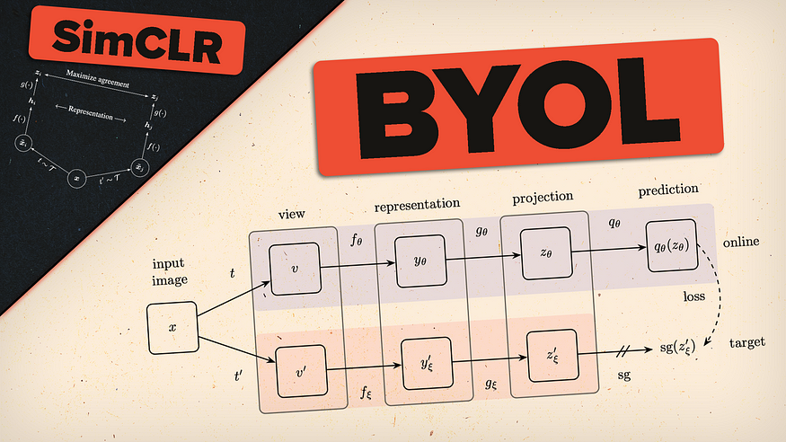
We can here see the exact idea that we have discussed so far! We have an input image and again produce two different views by applying two different sets of random augmentations. We use two different prediction paths, the online and target path, that make use of the same network architecture, but different sets of parameters. The target network’s parameters are an exponential moving average of the online network. What this more concretely means is that we update the target parameters by scaling its previous parameters by τ and adding the online networks parameters scaled by 1 — τ.

The authors, e.g., set τ=0.99, which means they only change the target parameters slightly, by adding the online parameters scaled by 0.01.

The Loss

Since we finally don’t have any contrastive examples anymore, we also don’t need a contrastive loss. The loss for BYOL is simply the Mean Squared Error between the normalized predictions and normalized target projections.

Well, that is almost the entire loss. As you can see, we are taking the loss between outputs of two different levels in each branch. Each pipeline, online and target, consists of the following networks. The representation network f, which we will use in downstream tasks, and a projection network g, as already seen in SimCLR! The online branch now further includes a prediction head q, which makes the entire architecture asymmetric between the online and target pipeline. What this means for the loss is that the authors symmetrize it by once feeding view v through the online and view v’ through the target network and a second time swapping the two views.

And that is the entire approach proposed in BYOL!

Results and Intuition

Training a ResNet50 using BYOL, and evaluating on ImageNet, of course, outperforms all other unsupervised baselines, including our previously discussed SimCLR, and comes surprisingly close to the fully supervised models!

This doesn’t mean, that BYOL always outperforms other models.

When pretraining on ImageNet and looking at Transfer learning results across different benchmarks, we can see that BYOL does not always perform the best! Also, it is interesting to see that the author’s report reproduced SimCLR results that perform better than those simply taken from the original paper. The authors don’t further elaborate on those findings and are not very consistent with when they use reproduced SimCLR and just referenced SimCLR results.

But that aside, they perform a deeper comparison with SimCLR! Arguably the most important reason, why we wanted an alternative to contrastive approaches such as SimCLR, was to reduce the sensitivity that comes with the reliance on negative samples.

When it comes to the effects of the batch size, the superiority of BYOL to SimCLR is obvious! BYOL is far less sensitive to smaller batch sizes than SimCLR. Which makes sense! When reducing the batch size to only 256 samples, BYOL’s top-1 accuracy only drops by 0.6%, while for SimCLR, it drops by 3.4%! The large drop that comes with reducing the batch size to 128 samples is hereby due to its effect on the batch normalization layer.

We have also already discussed how sensitive SimCLR is to the set of augmentations applied!

We can again see that BYOL is far less sensitive to the removal of important augmentations. In the end, when performing cropping only, the top-1 accuracy of BYOL drops by about 13%, while for SimCLR, it drops by about 28%! As already mentioned in my SimCLR post, this significant reliance on combining cropping with color jitter in the case of SimCLR is because, without the color augmentations, the model learns to simply differentiate histograms. Instead, BYOL is incentivized to keep any information captured by the target representation into its online network to improve its predictions. In other words, even if augmented views of the same image share the same color histogram, BYOL is still incentivized to retain additional features in its representation. For that reason, the authors at least believe that BYOL is more robust to the choice of image augmentations than contrastive methods.

The authors believe so? That’s really cool, and it obviously empirically works phenomenally. But why does it work? Why does it not collapse?
As mentioned, the authors don’t have mathematical proof, that this approach avoids collapse, but they have made a few empirical observations on what works and what doesn’t and hypothesize a few ideas as to why BYOL works.

Arguably the most important one is the addition of the predictor and ensuring that it is near-optimal. In fact, the authors hypothesize that the main role of BYOL’s target network is to ensure the near-optimality of the predictor over training. They have even found that they can completely remove the target network’s functionality without collapse by making the predictor near-optimal using other methods.

Let’s try to build some intuition! Remember, BYOL uses the projected representation z of this target network, whose weights are an exponential moving average of the weights of the online network, as a target for its online predictions using the additional predictor! This way, the weights of the target network represent a delayed and more stable version of the weights of the online network. The authors perform several ablation studies to develop an intuition of the importance of the right combination of the EMA target network and predictor.

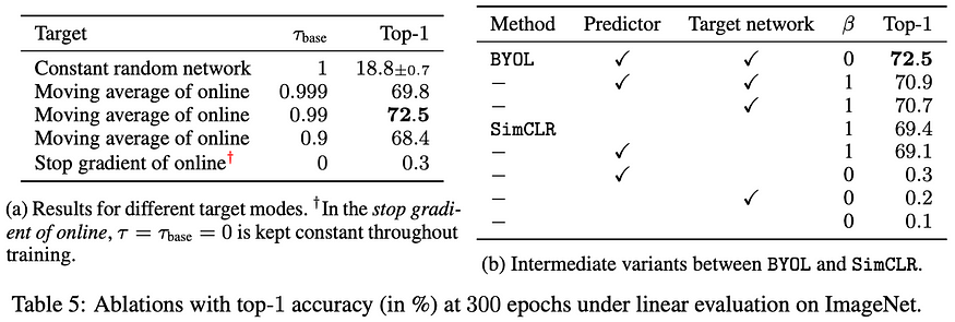
In the left table, we can see how the model performs under different EMA computations. The first case, τ = 1, is the exact experiment I described in the beginning, where the target network is a randomly initialized network, that is never updated. The last case, with τ = 0, describes the case where the target model is an exact copy of the online network, directly leading to a collapsed representation. The other cases just describe the search for the optimal τ parameter.
That said, it was later confirmed that the exponential moving average is not necessary. You can have the target network as a direct copy of the online network. That is if the predictor is updated more often or has a larger learning rate compared to the backbone. But it still provides training stability that can even somehow be used in SimCLR and actually boosts its performance.
Okay, the right table shows the effects of adding negative samples (second row), which hurts performance (!), and removing the predictor (third row), thus directly computing the loss between the projected representations of the online and target networks.
Nevertheless, all this does, in theory, still not completely avoid collapse. It just makes it “super difficult” and “unstable to get there”.

But okay, back to business. We’re almost done.
We have now understood how this new family of Self Supervised Learning works. We have had a look at BYOL, which is part of the Self-Distillation family that uses two neural networks, referred to as online and target networks, that interact and learn from each other. The great advantage of this approach is that it achieves great performance while not relying on negative pairs!

So, how can we further improve upon this idea? What technology has been taking over every domain of ML and is leading to amazing results?

[PAUSE]

Correct. Transformers.

We are now finally at the point where we can understand the apprach behind this visualization!

If you want to know how one of the most recent state-of-the-art models works, and what insights we can get from it have a look at the next post! We will cover the famous DINO paper by Mathilde Caron et. al., from Facebook AI Research!

And if it is not up yet, don’t forget to give me a follow to not miss the upload!

P.S.: If you like this content and the visuals, you can also have a look at my YouTube channel, where I post similar content but with more neat animations!

All Images are taken from the BYOL paper, created by the author with images the author has the rights to use, or by the referenced source.

Join thousands of data leaders on the AI newsletter. Join over 80,000 subscribers and keep up to date with the latest developments in AI. From research to projects and ideas. If you are building an AI startup, an AI-related product, or a service, we invite you to consider becoming a sponsor.

Published via Towards AI